This blog post describes how to train a Tensorflow Agents model. Before we start, we need a few things:

Table of Contents

Training description
1. Step 1
2. Step 2
3. Step 3
4. Repeat
Configuring the agent
Reply buffer
Training code
1. Why does it oscillate so much?

the environment in which the agent operates, it provides the observations, performs the actions selected by the agent and returns the reward. I am going to use the simplistic environment I wrote in this blog post.
a Tensorflow Agent driver to evaluate the performance of the agent. I will also use my custom metric, from this article.
the agent implementation, fortunately, that is provided by Tensorflow Agent, and we only need to configure it

Training description

Because reinforcement learning is not supervised learning, the training process is a little bit different. We have to train the neural network multiple times, and every iteration of training consists of three steps:

Step 1

First, we have to generate training examples by interacting with the environment using an epsilon greedy behavior policy (it means there is a \(1-\varepsilon\) probability of choosing the action returned by the neural network and \(\varepsilon\) probability of choosing a random action). It allows us to explore the solution space. I use the default value of the epsilon parameter, which gives me 10% of random data.

The generated examples are stored in a reply buffer. The reply buffer should be big enough to store examples from multiple iterations to give the neural network a diverse set of examples.

Step 2

We train the neural network using the data from the reply buffer as the input. The expected labels are generated by the previous version of the trained neural network.

It means that training loss metric has a different meaning. A low training loss indicates that the current iteration returns values similar to the previous one. To avoid getting stuck, we have the epsilon greedy behavior policy used for training set generation. We can also use an older version of the network to generate labels, but in this article, I am going to update the network in every iteration.

Step 3

We evaluate the trained agent by letting it interact with the environment. The environment returns the agent’s score (the reward). Obviously, our goal is to maximize the reward received by the agent.

Repeat

We repeat the above steps until we get a trained agent. Later, I will show you how to determine whether the training should be finished.

Configuring the agent

I am going to use, the Deep Q Network implementation, which was described in the “Human-level control through deep reinforcement learning” paper (Mnih et al., 2015). If you are not familiar with that research paper, I wrote a short article which explains that concept.

Tensorflow agents provide the implementation as the DqnAgent and QNetwork classes.

A QNetwork is a Feed-Forward neural network which approximates the Q function. The Q function returns the optimal behavior of the agent (the behavior that maximizes the expected reward).

I have a very simple environment, and I want to train the agent quickly, so I will give it a single hidden fully-connected layer of 100 neurons.

#tf_env is from the article mentioned at the beginning

import matplotlib.pyplot as plt
from tf_agents.agents.dqn import dqn_agent
from tf_agents.drivers import dynamic_step_driver
from tf_agents.networks import q_network
from tf_agents.replay_buffers import tf_uniform_replay_buffer

q_net = q_network.QNetwork(
    tf_env.time_step_spec().observation,
    tf_env.action_spec(),
    fc_layer_params=(100,))

agent = dqn_agent.DqnAgent(
    tf_env.time_step_spec(),
    tf_env.action_spec(),
    q_network=q_net,
    optimizer=tf.train.AdamOptimizer(0.001))

Reply buffer

As mentioned above, the reply buffer must be big enough to store examples from multiple training iterations.

replay_buffer = tf_uniform_replay_buffer.TFUniformReplayBuffer(
    agent.collect_data_spec,
    batch_size=tf_env.batch_size,
    max_length=10000)

Training code

Now, I can define the functions, which perform the steps of the training. First, I need a function that uses the epsilon greedy behavior policy to fill the reply buffer with training examples.

def collect_training_data():
  dynamic_step_driver.DynamicStepDriver(
    tf_env,
    agent.collect_policy,
    observers=[replay_buffer.add_batch],
    num_steps=1000).run()

After that, I define the function to train the neural network. The function also returns the loss in the current iteration.

def train_agent():
  dataset = replay_buffer.as_dataset(
      sample_batch_size=100,
      num_steps=2)

  iterator = iter(dataset)

  loss = None
  for _ in range(100):
    trajectories, _ = next(iterator)
    loss = agent.train(experience=trajectories)

  print('Training loss: ', loss.loss.numpy())
  return loss.loss.numpy()

The next function evaluates the neural network and returns the maximum reward.

def evaluate_agent():
  max_score = TFMaxEpisodeScoreMetric() # a class from the article mentioned at the beginning
  observers = [max_score]
  driver = dynamic_episode_driver.DynamicEpisodeDriver(
      tf_env, agent.policy, observers, num_episodes=100)

  final_time_step, policy_state = driver.run()

  print('Max test score:', max_score.result().numpy())
  return max_score.result().numpy()

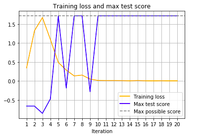
I run all three functions in a loop 20 times to train the agent and plot the chart of the maximal reward and training loss.

training_loss = []
max_test_score = []

for i in range(20):
  print('Step ', i)
  collect_training_data()
  training_loss.append(train_agent())
  max_test_score.append(evaluate_agent())

plt.plot(np.arange(1, 21, step = 1), training_loss, c = 'orange', label = 'Training loss')
plt.plot(np.arange(1, 21, step = 1), max_test_score, c = 'blue', label = 'Max test score')
plt.axhline(1.715, c = 'gray', linestyle='dashed', label = 'Max possible score')
plt.xlabel('Iteration')
plt.grid(True)
plt.title('Training loss and max test score')
plt.xticks(np.arange(1, 21))
plt.legend()

When the training finishes, we see that the returned reward eventually converged at a value that is also the maximal possible reward in that environment, so we have an optimally behaving agent.

We also see that when the agent reaches the maximum performance, the predictions returned by the neural network don’t differ from the ones returned by the previous version, so the training loss approaches zero.

Why does it oscillate so much?

My implementation of the environment is tricky. It gives the agent 0.1 rewards for every valid action (choosing an empty spot on the board), 1 for completing the board and -1 for attempting to make an illegal move (it also finishes the game). Hence it is easy to drop from 1.715 (the maximal discounted total reward in that environment) to -0.18, if the agent chooses 8 correct moves and makes a mistake in the last one.

How to train a Reinforcement Learning Agent using Tensorflow Agents

Training description

Step 1

Step 2

Step 3

Repeat

Configuring the agent

Reply buffer

Training code

Why does it oscillate so much?

How to use a custom metric with Tensorflow Agents

How to train a model in TensorFlow 2.0

How to train a Reinforcement Learning Agent using Tensorflow Agents

Training description

Step 1

Step 2

Step 3

Repeat

Configuring the agent

Reply buffer

Training code

Why does it oscillate so much?

How to use a custom metric with Tensorflow Agents

How to train a model in TensorFlow 2.0

Related Posts

Using Boltzmann distribution as the exploration policy in TensorFlow-agent reinforcement learning models

How to turn Pandas data frame into time-series input for RNN

How to automatically select the hyperparameters of a ResNet neural network