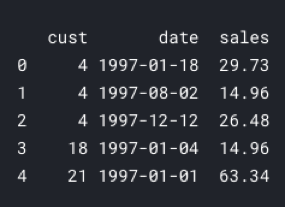
In this blog post, I am going to build a Pareto/NBD model to predict the number of customer visits in a given period. Such a model is the first part of predicting the customer lifetime value, but I am not going to use it for CLV prediction. I am going to focus on using it to predict customer churn. After all, if we see that the forecast for upcoming purchases is 0, we can send the customer a farewell message.

Table of Contents

Customer transactions
Cross-validation

First, we are going to need a list of customer transactions, but not all of them! The model works best if we split customers into cohorts and the input dataset contains only one cohort of customers.

import pandas as pd
import lifetimes
data = pd.read_csv("data.csv", header = 0)
data['date'] = pd.to_datetime(data['date'])

A cohort consists of all customers who made the first purchase in the same period. For example, we can get the transaction log of all customers who started buying our products in Q1 2018.

Customer transactions

In the second step, we must calculate a summary of the customer’s transaction log. We need three numbers calculated separately for every customer in the cohort. Those three numbers are:

recency — the time between the first and the last transaction
frequency — the number of purchases beyond the initial one
T — the time between the first purchase and the end of the calibration period

summary = lifetimes.utils.summary_data_from_transaction_data(data, 'cust', 'date')
summary = summary.reset_index()

To calculate the summary values, we are going to use the summary_data_from_transaction_data function from the lifetimes library. Note that, I did not specify the calibration period because I want to use all transactions from the input data frame. Also, the output is not going to be a standard RFM structure, because in this case, I am not interested in the monetary value, so I left this parameter out.

In the “lifetimes” implementation, the model has a penalizer_coef hyperparameter. I am not going to specify it in the first example, but in the second part of the blog post, I will show you how to split the transaction log into the training/test datasets. That will allow us to tune the hyperparameters.

Now, we can fit the model.

model = lifetimes.ParetoNBDFitter()
model.fit(summary['frequency'], summary['recency'], summary['T'])

After fitting the model, we can start predicting whether the customer is going to make another purchase. I need the summary metrics generated from the transaction log and the conditional_probability_alive function.

customer_id = 4

individual = summary[summary['cust'] == customer_id]
model.conditional_probability_alive(individual['frequency'], individual['recency'], individual['T'])

I promised that the model is going to predict customer churn, so we are not interested in the probability of being alive (which in this case mean: “the customer will buy something”), but the opposite of it:

1 - model.conditional_probability_alive(individual['frequency'], individual['recency'], individual['T'])

Cross-validation

The model we built in the first example may be incorrect. We can never be sure whether it gives us the correct values, because we have not tested it. To test the model, we must split the transaction log into the training and test (aka. holdout) datasets. We are going to build the model using the training set and then test its correctness using the test dataset.

Fortunately, in the lifetimes library that can be done using just two functions. Isn’t it convenient?

First, we must split the data.

from lifetimes.utils import calibration_and_holdout_data

summary_cal_holdout = calibration_and_holdout_data(
    data,
    'cust',
    'date',
    calibration_period_end=pd.to_datetime('1997-12-31'),
    observation_period_end=data['date'].max()
)

Now, we can build the model and tune its parameter.

model = lifetimes.ParetoNBDFitter(penalizer_coef=0.01)
model.fit(summary_cal_holdout['frequency_cal'], summary_cal_holdout['recency_cal'], summary_cal_holdout['T_cal'])

After that, we can forecast the customer purchases and compare the results with the real data from the holdout dataset.

from lifetimes.utils import expected_cumulative_transactions

freq = 'D' # days
number_of_days = 14

expected_vs_actual = expected_cumulative_transactions(model, holdout_set_transactions, 'date', 'cust', number_of_days, freq)

In machine learning, we asses the model performance by calculating one numeric value that describes the errors made by the model. I already have a dataset of actual and predicted values. Hence, I can calculate the RMSE:

from sklearn.metrics import mean_squared_error
from math import sqrt

sqrt(mean_squared_error(expected_vs_actual['actual'], expected_vs_actual['predicted']))

Predicting customer churn using the Pareto/NBD model

Customer transactions

Cross-validation

Business metrics that make no sense

Predicting customer lifetime value using the Pareto/NBD model and Gamma-Gamma model

Predicting customer churn using the Pareto/NBD model

Customer transactions

Cross-validation

Business metrics that make no sense

Predicting customer lifetime value using the Pareto/NBD model and Gamma-Gamma model

Related Posts

I worked as a data scientist and that was the worst job I have ever had.

How to remove outliers from Seaborn boxplot charts

Pandas stack and unstack explained