
How do we predict values of time series using recurrent neural networks in Tensorflow? Let’s try to predict how many people will read this blog on a given day.
Table of Contents
- Importing dependencies
- Loading the Dataset
- Data Exploration
- Outlier Detection
- Seasonality Detection
- Feature Engineering
- Feature Selection, Splitting the Dataset, and Normalization
- Splitting Data into Time Series
- Training a Model
- Getting the Results
- Results denormalization
Importing dependencies
Before we start, we should import all of the dependencies we will use later:
import pandas as pd
import numpy as np
import matplotlib.pyplot as plt

import requests

import tensorflow as tf
from tensorflow import keras
from tensorflow.keras import layers

from scipy.stats import zscore
Loading the Dataset
First, we have to download the dataset. I have put over a year of data on GitHub. In the file, we have dates and the number of people who read this website on that day:
r = requests.get('https://raw.githubusercontent.com/mikulskibartosz/RNN_workshop/main/visitors.csv%20-%20Sheet1.csv', allow_redirects=True)
with open('data.csv', 'wb') as f:
  f.write(r.content)

data = pd.read_csv('data.csv')
All of the values in the file are strings. For us, it is not a useful data type, so we must convert the columns to datetime and integers:
data['date'] = pd.to_datetime(data.date)

data['visitors'] = data['visitors'].str.replace(',', '')
data['visitors'] = data['visitors'].astype(int)
Data Exploration
In the beginning, we should take a look at the input data:
plt.rcParams["figure.figsize"] = (20,10)

plt.plot(data.date, data.visitors)
plt.xlabel('Date')
plt.ylabel('Number of visitors')
plt.title('The number of visitors between 2020.01.01 and March 2021')
plt.show()
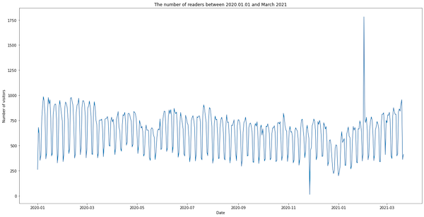
We see two peaks. The first one (the day with 13 visitors) happened when I made a mistake while updating the website template and accidentally removed the pageviews tracking code. The other peak (1781 visitors) occurred when someone was scrapping the website. We’ll remove both anomalies in the next section.
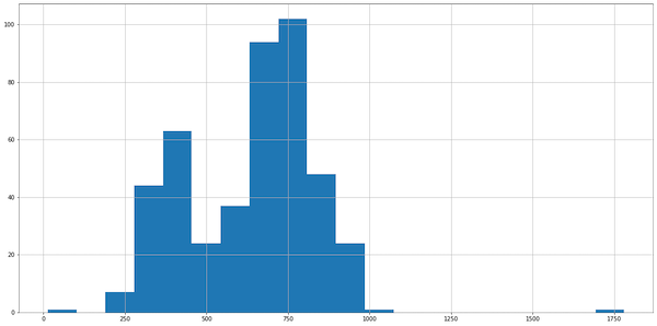
To complete data exploration, let’s take a look at a histogram:
data.visitors.hist(bins=20)
Outlier Detection
In the histogram, we see roughly Gaussian-ish distribution, so we can use the z-score to detect outliers. (Take a look at my other article if you want to know more about z-score and outlier detection):
visitor_zscores = zscore(data.visitors)
visitor_outliers = pd.Series(visitor_zscores).apply(
  lambda x: x <= -2.5 or x >= 2.5
)

data[visitor_outliers]
This code, correctly, finds the two outlier rows:
	date	visitors
331	2020-11-27	13
397	2021-02-01	1781
Removing Outliers
Because we have only two outliers, I suggest removing them by replacing the values with the average number of visitors on 2-3 days before and after the outlier:
data.loc[data['visitors'] == 1781, 'visitors']  = (641+763+728) / 3
data.loc[data['visitors'] == 13, 'visitors']  = (628 + 575 + 454 + 478) / 4
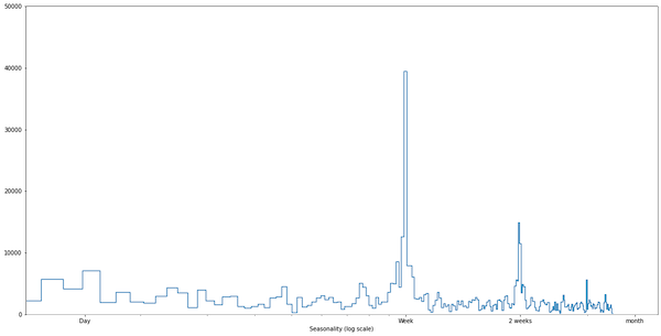
Seasonality Detection
When we look at the chart, we see seasonality: there are fewer visitors during the weekends. How can we prove that formally? For that, we can use the Fast Fourier Transform. It is a method of transforming a signal into its components (frequencies). We have to define a sampling frequency (in our case, a week) and plot frequencies. When we see a significant peak, we know that we have found seasonality:
fft = tf.signal.rfft(data['visitors'])
f_per_dataset = np.arange(0, len(fft))

n_samples_h = len(data['visitors'])
weeks_per_dataset = n_samples_h/(7) # because we use weeks for sampling

f_per_year = f_per_dataset/weeks_per_dataset # sampling frequency

plt.step(f_per_year, np.abs(fft))
plt.xscale('log')
plt.ylim(0, 50000)
plt.xlim([0.1, max(plt.xlim())])
plt.xticks([1.0/7, 1, 2, 4], labels=['Day', 'Week', '2 weeks', 'month'])
_ = plt.xlabel('Seasonality (log scale)')
Feature Engineering
Because we have found seasonality in one-week cycles, we have to pass a day of the week as one of the parameters. We’ll create three features. The first one indicates whether the day is a weekend day. The other two are sin and cos of the day number. I have written another article in which I explain why we encode days of the week in such a bizarre way.
data['day_of_week'] = data.date.dt.weekday
data['day_of_week_sin'] = np.sin(data['day_of_week'] * (2 * np.pi / 7))
data['day_of_week_cos'] = np.cos(data['day_of_week'] * (2 * np.pi / 7))
data['is_weekend'] = data['day_of_week'].isin([5, 6])
Feature Selection, Splitting the Dataset, and Normalization
Let’s select the features and split the dataset into training, validation, and test data.
features = data[['visitors', 'day_of_week_sin', 'day_of_week_cos', 'is_weekend']]

n = len(features)
train_df = features[0:int(n*0.7)]
val_df = features[int(n*0.7):int(n*0.9)]
test_df = features[int(n*0.9):]

num_features = features.shape[1]
Now, we have to normalize the data. During normalization, we subtract the average value of the training dataset from all datasets and divide the values by the training standard deviation. This is important! If we calculate the mean and standard deviation using also validation or test dataset, we will end up with data leakage. Data leakage during training happens when the model gets access to information it will not know in production.
train_mean = train_df.mean()
train_std = train_df.std()

train_df = (train_df - train_mean) / train_std
val_df = (val_df - train_mean) / train_std
test_df = (test_df - train_mean) / train_std
Splitting Data into Time Series
We can find a helpful class in the official Tensorflow time series tutorial. Let’s use it for converting datasets into time series in our code:
class WindowGenerator():
  def __init__(self, input_width, label_width, shift,
               train_df=train_df, val_df=val_df, test_df=test_df,
               label_columns=None):
    # Store the raw data.
    self.train_df = train_df
    self.val_df = val_df
    self.test_df = test_df

    # Work out the label column indices.
    self.label_columns = label_columns
    if label_columns is not None:
      self.label_columns_indices = {name: i for i, name in
                                    enumerate(label_columns)}
    self.column_indices = {name: i for i, name in
                           enumerate(train_df.columns)}

    # Work out the window parameters.
    self.input_width = input_width
    self.label_width = label_width
    self.shift = shift

    self.total_window_size = input_width + shift

    self.input_slice = slice(0, input_width)
    self.input_indices = np.arange(self.total_window_size)[self.input_slice]

    self.label_start = self.total_window_size - self.label_width
    self.labels_slice = slice(self.label_start, None)
    self.label_indices = np.arange(self.total_window_size)[self.labels_slice]

  def __repr__(self):
    return '\n'.join([
        f'Total window size: {self.total_window_size}',
        f'Input indices: {self.input_indices}',
        f'Label indices: {self.label_indices}',
        f'Label column name(s): {self.label_columns}'])

  def split_window(self, features):
    inputs = features[:, self.input_slice, :]
    labels = features[:, self.labels_slice, :]
    if self.label_columns is not None:
      labels = tf.stack(
        [labels[:, :, self.column_indices[name]] for name in self.label_columns],
        axis=-1)

    # Slicing doesn't preserve static shape information, so set the shapes
    # manually. This way the `tf.data.Datasets` are easier to inspect.
    inputs.set_shape([None, self.input_width, None])
    labels.set_shape([None, self.label_width, None])

    return inputs, labels

  def make_dataset(self, data):
    data = np.array(data, dtype=np.float32)
    ds = tf.keras.preprocessing.timeseries_dataset_from_array(
      data=data,
      targets=None,
      sequence_length=self.total_window_size,
      sequence_stride=1,
      shuffle=True,
      batch_size=32,)

    ds = ds.map(self.split_window)

    return ds

  @property
  def train(self):
    return self.make_dataset(self.train_df)

  @property
  def val(self):
    return self.make_dataset(self.val_df)

  @property
  def test(self):
    return self.make_dataset(self.test_df)

  @property
  def example(self):
    """Get and cache an example batch of `inputs, labels` for plotting."""
    result = getattr(self, '_example', None)
    if result is None:
      # No example batch was found, so get one from the `.train` dataset
      result = next(iter(self.train))
      # And cache it for next time
      self._example = result
    return result
Training a Model
To train the model, we’ll define a few more helper functions. First, we need a function to compile and train the model. It will accept the model configuration as a parameter, so we don’t have to copy/paste the training part of the code:
MAX_EPOCHS = 20

def compile_and_fit(model, window, patience=2):
  early_stopping = tf.keras.callbacks.EarlyStopping(monitor='loss',
                                                    patience=patience,
                                                    mode='min')

  model.compile(loss=tf.losses.MeanSquaredError(),
                optimizer=tf.optimizers.Adam(),
                metrics=[tf.metrics.MeanAbsoluteError()])

  history = model.fit(window.train, epochs=MAX_EPOCHS,
                      validation_data=window.val,
                      callbacks=[early_stopping])
  return history
Afterward, we define a training window. In this case, we want to pass 30 days to the model and get a prediction for the following two weeks:
data_window = WindowGenerator(
    input_width=30, label_width=14, shift=14,
    label_columns=['visitors'])
Model Definition and Training
Finally, we can write the model definition. We use two layers of LSTM neurons with Dropout to prevent overfitting. The last two layers transform the output into the final result:
lstm_model = tf.keras.Sequential([
    tf.keras.layers.LSTM(256, return_sequences=True),
    tf.keras.layers.Dropout(0.4),
    tf.keras.layers.LSTM(256, return_sequences=False),
    tf.keras.layers.Dropout(0.4),
    tf.keras.layers.Dense(14*num_features,
                          kernel_initializer=tf.initializers.zeros()),
    tf.keras.layers.Reshape([14, num_features])
])

compile_and_fit(lstm_model, data_window)
Getting the Results
In the last step, we’ll use the test dataset to predict the number of visitors and compare the prediction with the actual results. We’ll need an additional function to display a chart with the results:
def plot(window, model=None, plot_col='visitors'):
    inputs, labels = window.example
    plt.figure(figsize=(12, 8))
    plot_col_index = window.column_indices[plot_col]

    plt.ylabel(f'{plot_col} [normed]')
    plt.plot(window.input_indices, inputs[0, :, plot_col_index],
            label='Inputs', marker='.', zorder=-10)

    if window.label_columns:
      label_col_index = window.label_columns_indices.get(plot_col, None)
    else:
      label_col_index = plot_col_index

    plt.scatter(window.label_indices, labels[0, :, label_col_index],
                edgecolors='k', label='Labels', c='#2ca02c', s=64)
    if model is not None:
      predictions = model(inputs)
      plt.scatter(window.label_indices, predictions[0, :, label_col_index],
                  marker='X', edgecolors='k', label='Predictions',
                  c='#ff7f0e', s=64)

      plt.legend()

    plt.xlabel('Days')
When we have the function, we can plot the results:
plot(data_window, lstm_model)
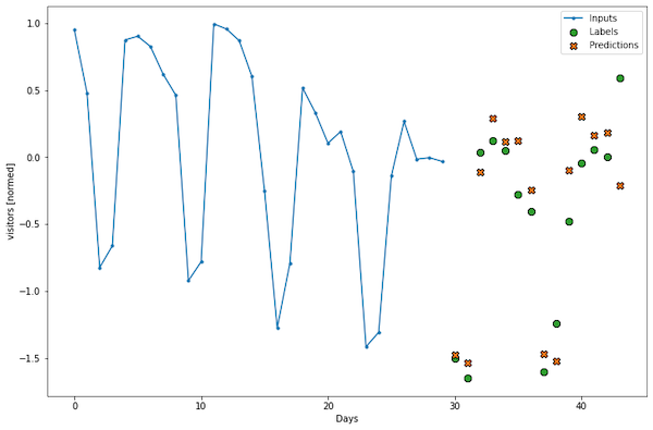
Is this a good result? When we look at the mean absolute error of validation set prediction, we see 0.6619 (your value may differ a little bit). I think we can make it better. However, finding better hyperparameters is tricky, so the right solution here is to use Keras Tuner to automate it. Here are my other articles about Keras Tuner:
- Using Keras Tuner to tune hyperparameters in Tensorflow
- Using Hyperband algorithm in Keras Tuner
- How to automatically select hyperparameters of a ResNet model
Results denormalization
Have you noticed that the prediction is normalized? If we need the actual predicted number, we have to denormalize the result:
denomralized_prediction = normalized_model_prediction * train_std + train_mean