
Regression
Regression predicts a quantity (a number where “bigger” and “closer” mean something). The inputs can be anything: numbers, categories, text. It’s the answer that has to be a measurement. (When the answer is a category instead, that’s classification, and we’ll get there.)
In the regression part of the book, we use the “MPG dataset.” If you followed any ML tutorial, you have probably used it. Everyone has seen this dataset and almost nobody has looked at it. The dataset contains features describing a car model, and the target variable MPG, which means miles per gallon. Given the available attributes of a vehicle, we will attempt to predict how many miles it can drive on a single gallon of gasoline. Here are the first five rows of that dataset.
import matplotlib.pyplot as plt
import pandas as pd
import numpy as np

data_url = "https://archive.ics.uci.edu/ml/machine-learning-databases/auto-mpg/auto-mpg.data"
column_names = ['mpg', 'cylinders', 'displacement', 'horsepower', 'weight', 'acceleration', 'model year', 'origin', 'car name']
df = pd.read_csv(data_url, sep=r"\s+", names=column_names)
df.head()
| mpg | cylinders | displacement | horsepower | weight | acceleration | model year | origin | car name |
|---|---|---|---|---|---|---|---|---|
| 18 | 8 | 307 | 130 | 3504 | 12 | 70 | 1 | chevrolet chevelle malibu |
| 15 | 8 | 350 | 165 | 3693 | 11.5 | 70 | 1 | buick skylark 320 |
| 18 | 8 | 318 | 150 | 3436 | 11 | 70 | 1 | plymouth satellite |
| 16 | 8 | 304 | 150 | 3433 | 12 | 70 | 1 | amc rebel sst |
| 17 | 8 | 302 | 140 | 3449 | 10.5 | 70 | 1 | ford torino |
What do we know about this dataset? The dataset alone doesn’t say much, we will need to find some documentation. MPG is an old dataset and multiple versions exist, so it’s difficult to find documentation for the exact version you happen to download. The page I linked to documents a different one, and not only in formatting: it lists origin as named regions instead of the numbers 1, 2, 3, writes the model year as 1970-1982 instead of 70-82, and has 392 rows where ours has 398. The missing six are the rows with an unknown horsepower value, which somebody had already removed from that version. In other words, the documentation describes a dataset in which the problem we are about to find does not exist. Good for a simple working example, not so good for teaching how to debug problems.1
-
mpg: how far the car travels on one gallon, measured in miles -
cylinders: the number of cylinders in the engine -
displacement: the engine’s displacement measured in cubic inches -
horsepower: the engine power, obviously (or… not so obviously?) -
weight: the car’s weight in pounds -
acceleration: the time from 0 mph to 60 mph, measured in seconds -
model year: the model year, 70 means 1970, and so on -
origin: the region of origin. In this dataset 1 = USA, 2 = Europe, and 3 = Japan -
car name: the make and the model name
The target variable is the variable we choose to predict. Nothing in the dataset forces us to predict MPG. We could decide to predict the horsepower or the model name2, given all other independent variables. In practice, we often know in advance what we want to predict and then gather data required to make such predictions. In our example, the question we want to answer may be: “given a car that weighs 3,500 lbs, has 8 cylinders and 150 hp, what mpg should I expect?”
One more thing about the target variables: you can also see names such as target feature, dependent variable, label, or just y. They all mean the same thing. It’s the value we want to predict using the model.
An independent feature or an independent variable (also called predictors, inputs, or X) is the value we use to predict the target variable. The assumption is that, when we use the trained model on real data, we know the independent variables, but don’t know the target variable. Also, the “independent” adjective is a bit of a lie in practice. The features are usually correlated with each other. Even in this dataset, we will see that heavier cars tend to have more cylinders, bigger displacement, and bigger horsepower.3
How do you know anything I just said about this data is true? You don’t. Now it’s time to look at the data, verify the range and distribution of values, seek missing values, mixed-up units of measurement, and tons of other problems.
As a person who spent a substantial part of my career doing data engineering, I beg you to never ever trust any dataset. I remember a data engineering project where our main pipeline failed due to a source API change, so the replacement pipeline was writing data to a temporary location. The data engineer assigned to review the PR didn’t read the Jira ticket, assumed the temporary location contained test data, and deleted it. We lost a week of production data. Don’t trust data engineers (especially if you are one).
Sometimes, data engineers update the pipeline code and forget to run a backfill4, or decide to never do it, but that decision isn’t documented anywhere. Data formats change, units of measurement change. What stays the same is the documentation that was written three years ago by someone who didn’t understand the business domain and that never got updated.
Examining the data
Even in this toy dataset, there are traps. Here is how we prove the data is correct or find the issues before our training code crashes, or, worse, we successfully train a model that makes no sense.
We will start with the boring, but still important, stuff we have to check before we continue. First, how many values did we load?
df.shape
# (398, 9)
# explanation: the first value is the number of rows, the second the number of columns
The source page promises 398 instances, so that looks correct, but the dataset description says we have seven features, and we have nine columns. What happened? The target variable is often not counted as a feature. What about the ninth column? The description claims the car name is an ID column, not a feature. That makes nine columns in total.
We have already looked at the first five rows above and everything looked fine. The values loaded correctly. Did they? We have eight numeric columns and one text (in pandas, denoted as the type called object). Let’s confirm it by reading the df.dtypes field:
| 0 | |
|---|---|
| mpg | float64 |
| cylinders | int64 |
| displacement | float64 |
| horsepower | object |
| weight | float64 |
| acceleration | float64 |
| model year | int64 |
| origin | int64 |
| car name | object |
Why is horsepower an object? We need to check which rows don’t contain a valid number in the horsepower column.
Finding missing values
df[pd.to_numeric(df['horsepower'], errors='coerce').isna()]['horsepower']
| horsepower | |
|---|---|
| 32 | ? |
| 126 | ? |
| 330 | ? |
| 336 | ? |
| 354 | ? |
| 374 | ? |
What are question marks doing here? Apparently, missing values are denoted with “?” Where does the dataset description mention it? You guessed it: nowhere (they just mention there are some missing values, with no additional information). We have just found the first trap in this dataset. Are there any others? Let’s reload the dataset while replacing “?” with a None type, and keep looking.
df = pd.read_csv(data_url, sep=r"\s+", names=column_names, na_values="?")
# if you use df.dtypes again, you will see that horsepower is now a float, so we corrected the problem
Right now, we should see those six missing numbers in our dataset. Let’s confirm it and, at the same time, check if there are more missing values.
df[df.isnull().any(axis=1)]
| mpg | cylinders | displacement | horsepower | weight | acceleration | model year | origin | car name | |
|---|---|---|---|---|---|---|---|---|---|
| 32 | 25 | 4 | 98 | nan | 2046 | 19 | 71 | 1 | ford pinto |
| 126 | 21 | 6 | 200 | nan | 2875 | 17 | 74 | 1 | ford maverick |
| 330 | 40.9 | 4 | 85 | nan | 1835 | 17.3 | 80 | 2 | renault lecar deluxe |
| 336 | 23.6 | 4 | 140 | nan | 2905 | 14.3 | 80 | 1 | ford mustang cobra |
| 354 | 34.5 | 4 | 100 | nan | 2320 | 15.8 | 81 | 2 | renault 18i |
| 374 | 23 | 4 | 151 | nan | 3035 | 20.5 | 82 | 1 | amc concord dl |
Six rows and all missing values are in the horsepower column (nan means “not a number”). Good, but what do we do now? We have three options: we can remove the rows with missing values, replace those values with a value of our choice, or just keep them5 in the current form. I have a separate chapter about dealing with missing values in the classification section (as the example dataset used there gives us more options), so for now we will drop them and pretend this is the best we can do (it isn’t the best solution, by the way).
df = df.dropna()
# removing rows where any value is missing
Checking the range of values
We have some expectations regarding all values. First of all, we shouldn’t see any zero or negative values. If we see a magical car that produces fuel while driving (a negative mpg), we would need to go back a step and verify the process that produced the dataset.
At this point, when we look at the dataset summary statistics (df.describe()), we care about the minimum and the maximum values:
| mpg | cylinders | displacement | horsepower | weight | acceleration | model year | origin | |
|---|---|---|---|---|---|---|---|---|
| count | 392 | 392 | 392 | 392 | 392 | 392 | 392 | 392 |
| mean | 23.4459 | 5.47194 | 194.412 | 104.469 | 2977.58 | 15.5413 | 75.9796 | 1.57653 |
| std | 7.80501 | 1.70578 | 104.644 | 38.4912 | 849.403 | 2.75886 | 3.68374 | 0.805518 |
| min | 9 | 3 | 68 | 46 | 1613 | 8 | 70 | 1 |
| 25% | 17 | 4 | 105 | 75 | 2225.25 | 13.775 | 73 | 1 |
| 50% | 22.75 | 4 | 151 | 93.5 | 2803.5 | 15.5 | 76 | 1 |
| 75% | 29 | 8 | 275.75 | 126 | 3614.75 | 17.025 | 79 | 2 |
| max | 46.6 | 8 | 455 | 230 | 5140 | 24.8 | 82 | 3 |
We see no negative values and no unrealistically high values. It also seems that the units are consistent because if we had displacement with cubic inches and cubic centimeters mixed up, we would see values over 1,000. The only column that may still contain mixed-up units is weight, as the min and max values are plausible for both kilograms and pounds (we will verify it with a histogram in a second).
The dataset contains three more columns we need to verify: cylinders, origin, and model year. All three are currently numbers. Integers, as we have seen while reading dtypes. At least, we know there are no cars with 3.5 cylinders. However, we expect to see every number in the ranges 3-8 cylinders (with 7 missing because nobody has ever mass-produced a car with 7 cylinders), 1-3 origin, and 70-82 in the model year column. We can verify it by looking at the available unique values:
print(f"Unique values for 'cylinders': {sorted([int(x) for x in df['cylinders'].unique()])}")
print(f"Unique values for 'origin': {sorted([int(x) for x in df['origin'].unique()])}")
print(f"Unique values for 'model year': {sorted([int(x) for x in df['model year'].unique()])}")
# Unique values for 'cylinders': [3, 4, 5, 6, 8]
# Unique values for 'origin': [1, 2, 3]
# Unique values for 'model year': [70, 71, 72, 73, 74, 75, 76, 77, 78, 79, 80, 81, 82]
Every value is in range. Origin and model year are fine. But look at the cylinders again, and not at the 7 that isn’t there. Look at the 3 that is.
df[df['cylinders'] == 3][['car name', 'displacement', 'horsepower', 'mpg', 'model year']]
| mpg | cylinders | displacement | horsepower | weight | acceleration | model year | origin | car name | |
|---|---|---|---|---|---|---|---|---|---|
| 71 | 19 | 3 | 70 | 97 | 2330 | 13.5 | 72 | 3 | mazda rx2 coupe |
| 111 | 18 | 3 | 70 | 90 | 2124 | 13.5 | 73 | 3 | maxda rx3 |
| 243 | 21.5 | 3 | 80 | 110 | 2720 | 13.5 | 77 | 3 | mazda rx-4 |
| 334 | 23.7 | 3 | 70 | 100 | 2420 | 12.5 | 80 | 3 | mazda rx-7 gs |
Four cars, and all four are Mazdas: the RX-2, the RX-3 (misspelled “maxda rx3” in this file), the RX-4, and the RX-7. Those cars don’t have 3 cylinders. They don’t have cylinders at all. They are Wankel rotaries, their engines have rotors6, and whoever assembled this dataset needed an integer for a column that doesn’t apply to those cars, so they wrote 3.
Our data range check passed and the answer is still wrong. That is the failure mode a range check cannot catch: the value sits inside the allowed set, it looks plausible, and it means nothing. It also contaminates a second column, because rotary chamber volume isn’t measured the way piston displacement is. That’s why a 70-cubic-inch engine in this dataset makes 97 hp. Remember it when we interpret the coefficient on cylinders.
One more thing. We don’t see that problem in our dataset, but sometimes people have the idea of using a sentinel value instead of a missing value. We had “?” in a numeric column, which is sort of a sentinel value, but it could be way worse. At least in our case, the sentinel had an unexpected type (a string instead of a number). Occasionally, you may see a dataset where a missing positive number is denoted with -1, -999, or whatever abomination the author chose instead of just using a null. Or a date from a “distant future” to mark a missing date. Obviously, that “distant future” is already in the past on the day you read the dataset. Nulls may be Tony Hoare’s billion-dollar mistake, but whatever this “cleverness” is, it’s 10x worse. Don’t do it, and watch out for it in the data you receive.
We have seen both ends of value ranges and they looked correct. However, we also have some expectation about the data distribution. We already checked the small ranges of very specific integer values and found one that passed the check while being wrong anyway. But there is more:
-
mpg: the dataset pools 13 model years, and the efficiency gains arrived gradually across them (we will discuss that soon), so the genuinely economical cars are a thin slice concentrated at the end while the bulk of the fleet sits in the ordinary range. Values can’t run below zero either (no car does worse than zero miles per gallon) and mpg has no ceiling (I hope, every time I fuel my car), so the spread has nowhere to go but up. Expect lots of ordinary cars and a handful of efficient ones. -
displacementandhorsepowershould form a multimodal (not a single peak, but a few of them) histogram as we should see different engine families. -
weightgrouped by origin should not show European and Japanese values around 2.2× smaller than US because it could mean their weights are written in kilograms instead of pounds.
mean_mpg = df['mpg'].mean()
median_mpg = df['mpg'].median()

plt.figure(figsize=(10, 6))
plt.hist(df['mpg'], bins=30, edgecolor='black', alpha=0.7, label='MPG Distribution')

plt.axvline(mean_mpg, color="#4d41e0", linestyle='--', linewidth=2, label=f'Mean MPG: {mean_mpg:.2f}')
plt.axvline(median_mpg, color="#eb6834", linestyle='-.', linewidth=2, label=f'Median MPG: {median_mpg:.2f}')

plt.title('Distribution of MPG with Mean and Median', loc='left')
plt.xlabel('Miles Per Gallon (MPG)')
plt.ylabel('Frequency')
plt.grid(axis='y', alpha=0.75)
plt.legend()
plt.show()
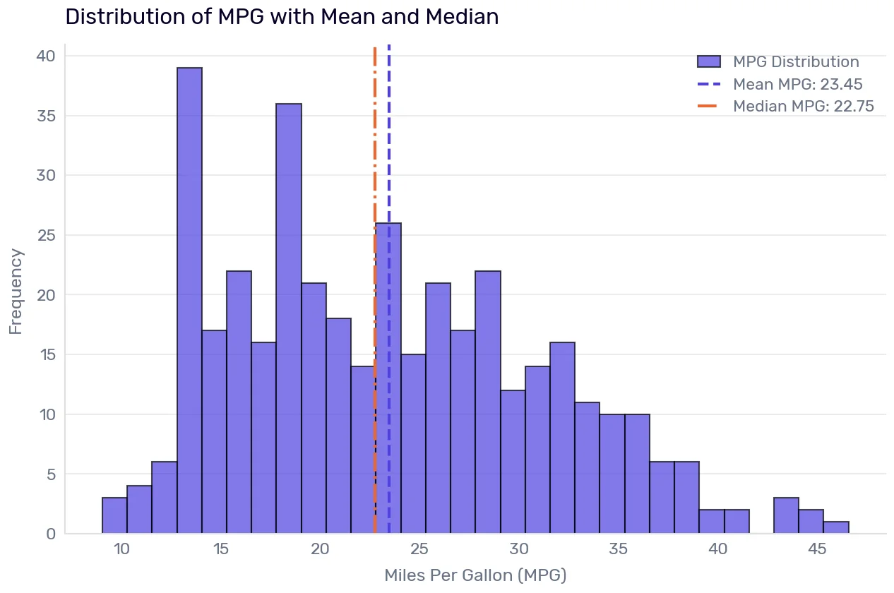
Right-skewed, as expected (mildly, but measurably). The mean (23.45) sits above the median (22.75), which is exactly what a long right tail does: a handful of very economical cars drag the average up while most of the fleet clusters lower. That gap between mean and median is the cheapest skew detector you have.
fig, axes = plt.subplots(nrows=2, ncols=1, figsize=(10, 12))

# Histogram for Displacement
axes[0].hist(df['displacement'], bins=30, edgecolor='black', alpha=0.7)
axes[0].set_title('Distribution of Displacement', loc='left')
axes[0].set_xlabel('Displacement')
axes[0].set_ylabel('Frequency')
axes[0].grid(axis='y', alpha=0.75)

# Histogram for Horsepower
axes[1].hist(df['horsepower'], bins=30, edgecolor='black', alpha=0.7)
axes[1].set_title('Distribution of Horsepower', loc='left')
axes[1].set_xlabel('Horsepower')
axes[1].set_ylabel('Frequency')
axes[1].grid(axis='y', alpha=0.75)

plt.tight_layout()
plt.show()
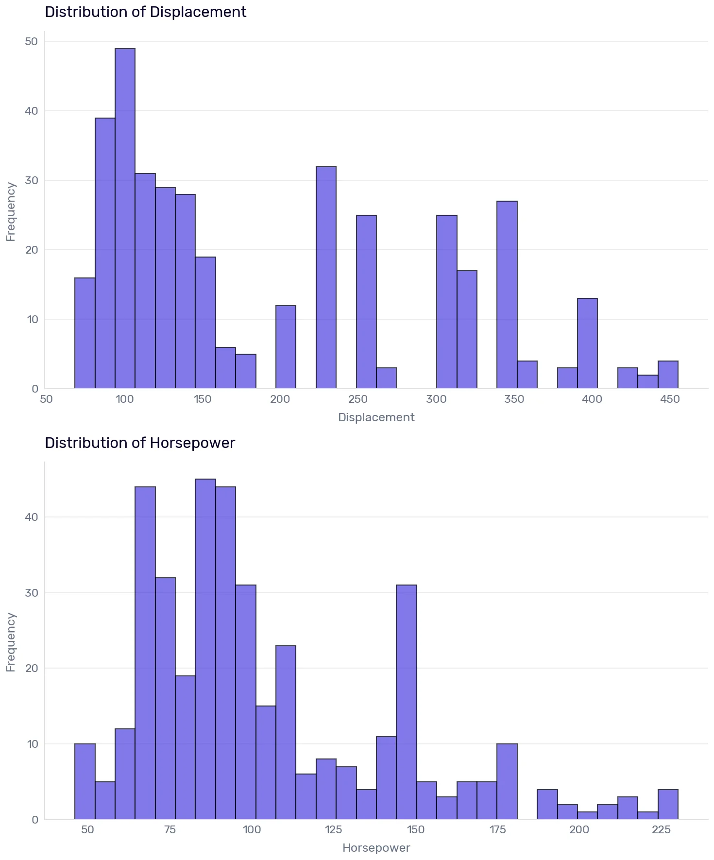
As expected, we see multiple engine families in the horsepower and displacement histograms. Now, the last column where we expect a problem.
ORIGIN_NAMES = {1: "USA", 2: "Europe", 3: "Japan"}
SERIES = ["#4d41e0", "#eb6834", "#1baf7a", "#e87ba4", "#eda100", "#008300"]

plt.figure(figsize=(10, 6))

for origin_code, origin_name in ORIGIN_NAMES.items():
    origin_data = df[df['origin'] == origin_code]

    plt.hist(origin_data['weight'], bins=30, alpha=0.6,
             label=origin_name, edgecolor='black',
             color=SERIES[origin_code - 1])

plt.title('Distribution of Weight by Origin', loc='left')
plt.xlabel('Weight (lbs, hopefully)')
plt.ylabel('Frequency')
plt.grid(axis='y', alpha=0.75)
plt.legend(title='Origin')
plt.show()
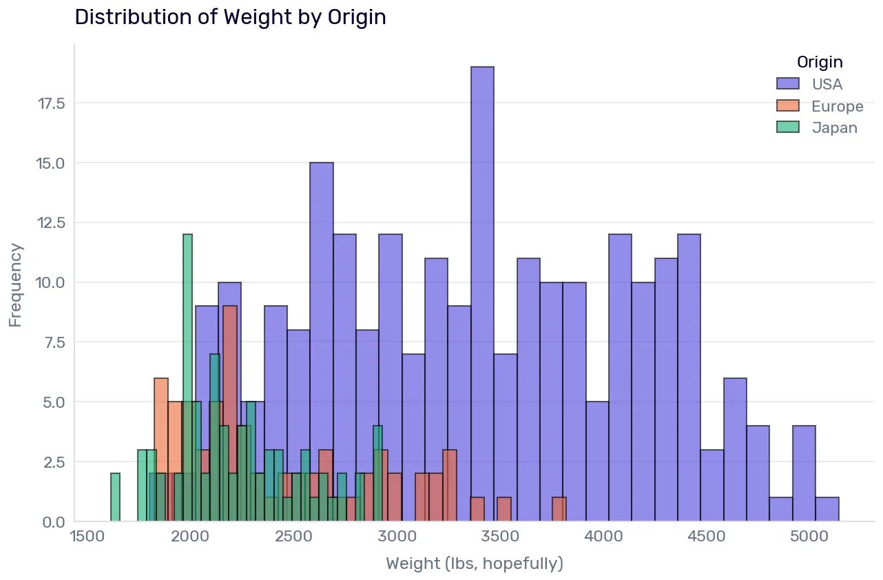
Not the 2.2× gap that would mean kilograms. The Japanese and European bulk sits about 1.5× lighter than the American, which is roughly what you would expect from the actual cars. But “roughly what I expected” is a feeling, not a check. So let’s get an external source of truth. I will use the Automobile Catalog to find the car’s data and compare with the value we have in our dataset. I will pick two European and two Japanese cars7 (the light ones), and if we see more or less the same value (small differences are allowed because we may compare different variants of the same car) in the Automobile Catalog, we assume we measure weights in pounds in all cases.
| displacement | car name | model year | weight | AC weight |
|---|---|---|---|---|
| 131 | audi 5000 | 78 | 2830 | 2859 |
| 68 | fiat 128 | 73 | 1867 | 1835 |
| 85 | datsun f-10 hatchback | 77 | 1945 | 1971 |
| 113 | toyota corona mark ii | 70 | 2372 | 2249 |
It seems all weight values are in pounds.
Numbers that aren’t numbers and other tricky columns
We have three numeric columns that need special attention. The most obvious is origin as it isn’t really a number. US + Europe = Japan? In our dataset, apparently, yes. Origin is a categorical variable that happens to be encoded as a number. We will need to transform it into multiple columns, so the ML algorithm can distinguish between values without the implicit assumption that one is greater/smaller than another. However, our first attempt to train the model will ignore that fact, so you can observe what happens when you make a mistake by using a categorical variable as a number.
Cylinders are numbers, integers to be precise. No car with 4.3 cylinders can exist. If we ever used that model in production, we would need to validate the input data. For our purposes, we must remember the set of possible values, so we don’t say anything stupid when we interpret the model.
Acceleration is a number, decimal values are allowed. So what’s so special about it? The value tells us how many seconds the car needs to accelerate from 0 mph to 60 mph. The bigger the value, the worse it is. Not a problem for ML models, but again, we need to remember that fact while interpreting the model coefficients.
The car name is another special column. The dataset description denotes it as the ID, so we expect mostly unique values (with the exception of the same model released in different variants across multiple years). That near-uniqueness is what makes it unusable as a feature in its current form. However, the name consists of the car’s make and model. Later, we will extract the make and use it as a feature. For now we ignore the column.
Duplicates
Our dataset contains no exact duplicates (you can confirm it by running df.duplicated().sum(), and note that this checks entire rows). Usually, we want the dataset to contain only unique records. In particular, we don’t want the same record to occur in both the training and test dataset. That’s called data leakage and we will talk about it in the next chapter.
Be careful before reaching for drop_duplicates(), though. There’s a difference between a duplicate record (one real thing accidentally recorded twice) and two genuinely different things that happen to have identical measurements. Two different customers can be the same age, earn the same salary, and live in the same city. Dropping the second kind throws away real information about how common those values are.
Finally, some ML models support an additional sample weight parameter denoting the importance of a data sample, so instead of dropping duplicates you can count them and instruct the model to “pay more attention” to the ones that repeat.
One more case worth knowing: identical features but a different target value. That is not a duplicate to delete. It’s noise you cannot remove, and it tells you the ceiling on how accurate any model can get on this data.
Cross-checking the data against business knowledge
Checking whether the range of values looks like we expect or whether some values are missing is important, but it won’t help us answer the most critical question: is this data true? What’s the data lineage? Where did it come from? How was it preprocessed before we got it?
According to the UC Irvine page, our version is a modified version of the dataset from the CMU StatLib library, used in 1993 by Ross Quinlan in a research paper, and the only modification was removing the rows with empty mpg values. Was the dataset in the CMU StatLib library correct? We don’t know. We will never be sure, but we can run a few checks.
Knowing the business domain (or googling for 5 minutes), we can expect to observe two events in this dataset:
- The horsepower for the cars produced by the US manufacturers should drop sharply in 1972 because they switched from SAE gross to SAE net horsepower ratings.
- The 1973 Oil Crisis should be visible in the dataset: smaller engines and more miles per gallon.
But… let’s start smaller. Can we trust the origin column? Let’s check if the car models look plausible:
for origin_code, origin_name in ORIGIN_NAMES.items():
    print(f"\nOrigin: {origin_name} (Code: {origin_code})")
    cars_by_origin = df[df['origin'] == origin_code]['car name']
    for car_name in cars_by_origin.head(3):
        print(f"- {car_name}")
Origin: USA (Code: 1)
- chevrolet chevelle malibu
- buick skylark 320
- plymouth satellite

Origin: Europe (Code: 2)
- volkswagen 1131 deluxe sedan
- peugeot 504
- audi 100 ls

Origin: Japan (Code: 3)
- toyota corona mark ii
- datsun pl510
- datsun pl510
Chevrolet in the US, Volkswagen, and Peugeot in Europe, Toyota in Japan. The origin column looks fine. Of course, we should check every value, but let’s be serious: you don’t want to look at a table with 400 rows while reading a book, do you? (When you work with production data, sample the values and at least skim them.)
Now, the rating change. Let’s divide horsepower by displacement, giving us horsepower per cubic inch. We do this because engines were also getting smaller across these years. If we plotted raw horsepower, a drop could mean the rating convention changed or the engines shrank, and we couldn’t tell which. Per cubic inch, engine size is held roughly constant, so a drop points to the switch to a different rating. We expect to see a 20% drop in the US ratings between 1971 and 1972.
df["hp_per_cid"] = df["horsepower"] / df["displacement"]
median_hp_per_cid = df.groupby(['model year', 'origin'])['hp_per_cid'].median().unstack()

fig, ax = plt.subplots()
for origin_code, color in zip(ORIGIN_NAMES.keys(), SERIES):
    if origin_code in median_hp_per_cid.columns:
        ax.plot(median_hp_per_cid.index, median_hp_per_cid[origin_code], color=color, label=ORIGIN_NAMES[origin_code], marker='o', markeredgecolor="#ffffff", markeredgewidth=1.5)

ax.set_title("Median Horsepower per Cubic Inch by Model Year and Origin")
ax.set_xlabel("Model Year")
ax.set_ylabel("Median Horsepower per Cubic Inch")
ax.set_ylim(bottom=0)
ax.legend(title="Origin", loc="upper left", bbox_to_anchor=(1.02, 1))

# The year when we expect to see a drop in the horsepower of US cars
ax.axvline(x=72, linestyle=':', color='red', alpha=0.4)

# If we are right, the values should be below this line
value_year_71_origin_1 = median_hp_per_cid.loc[71, 1]
horizontal_line_value = value_year_71_origin_1 * 0.8
ax.axhline(y=horizontal_line_value, linestyle='--', color='gray', alpha=0.6)

plt.tight_layout()
plt.show()
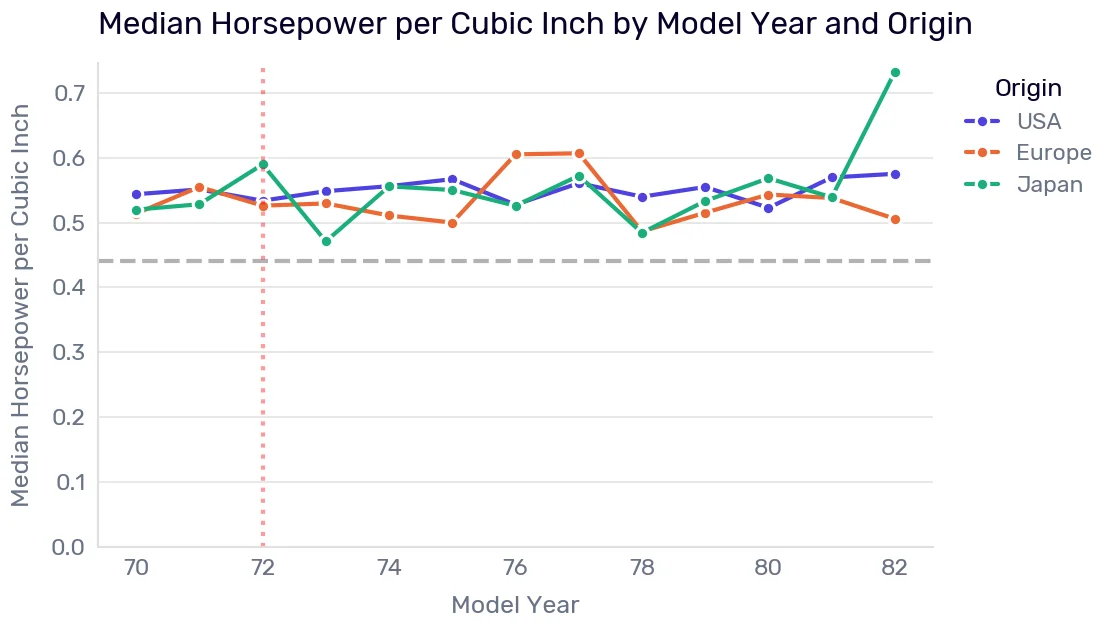
Not even close. What happened? Let’s look at the 1970 Chevelle 307 data row and its Automobile Catalog page.
| mpg | cylinders | displacement | horsepower | weight | acceleration | model year | origin | car name |
|---|---|---|---|---|---|---|---|---|
| 18 | 8 | 307 | 130 | 3504 | 12 | 70 | 1 | chevrolet chevelle malibu |
The page says the car’s horsepower was 200 hp (SAE gross), we have 130 hp. Perhaps our dataset was already converted to SAE net. Perhaps nobody documented such a conversion, or perhaps the record was not preserved over the years and subsequent versions of this dataset.
Our dataset says the car weighs 3504 lbs, and according to the Automobile Catalog it weighs 3413 lbs. A tiny difference. We could let it slide. However, our acceleration column claims the car needs 12 s to get from 0 mph to 60 mph. The Automobile Catalog: 10.1 s. But… the catalog describes a specific version of that Chevelle Malibu. Our dataset, too. But we have no clue which one.
Let’s look at a 1973 Plymouth Duster 198. Horsepower? Same. Weight? Similar enough (2904 vs. 2921 lbs). Acceleration? Same. MPG? Noticeably different (23 mpg vs. 18.1).
| mpg | cylinders | displacement | horsepower | weight | acceleration | model year | origin | car name |
|---|---|---|---|---|---|---|---|---|
| 22 | 6 | 198 | 95 | 2833 | 15.5 | 70 | 1 | plymouth duster |
| 23 | 6 | 198 | 95 | 2904 | 16 | 73 | 1 | plymouth duster |
| 20 | 6 | 198 | 95 | 3102 | 16.5 | 74 | 1 | plymouth duster |
Hypothesis 1 fails, and the failure is the finding. Look at the Duster rows again: the same 198-cubic-inch engine reads 95 hp in 1970 and 95 hp in 1973, on either side of the SAE switch. We expect the gross SAE rating to be systematically higher than the net rating for the same engine. Our 1970 row already holds the net figure!
That is why the chart above is flat.8 The horsepower column didn’t drop in 1972 because somebody had already converted it before this dataset reached us, but they didn’t write that down.
Two rows are an anecdote, though, so let’s check every model9 that appears on both sides of the change:
us_cars = df[df["origin"] == 1]
spanning = (
    us_cars.assign(era=np.where(us_cars["model year"] < 72, "pre-72", "72+"))
      .groupby(["car name", "displacement", "era"])["horsepower"]
      .median()
      .unstack("era")
      .dropna()
)
spanning["change_pct"] = (spanning["72+"] / spanning["pre-72"] - 1) * 100
spanning.sort_values("change_pct")
| 72+ | pre-72 | change_pct | |
|---|---|---|---|
| (‘ford maverick’, 200.0) | 81 | 85 | -4.70588 |
| (‘amc gremlin’, 232.0) | 100 | 100 | 0 |
| (‘chevrolet impala’, 350.0) | 165 | 165 | 0 |
| (‘ford galaxie 500’, 351.0) | 153 | 153 | 0 |
| (‘plymouth duster’, 198.0) | 95 | 95 | 0 |
| (‘plymouth fury iii’, 318.0) | 150 | 150 | 0 |
If the ratings had changed convention mid-dataset, these pairs would cluster around a 20% drop. Almost all of them don’t change at all, and in the case of the one that changes, the difference isn’t dramatic.
We also noticed our values don’t match the Automobile Catalog. Is at least one of the sources wrong? Or are we comparing two variants of the same car? We will never know, because the rows aren’t specific enough to identify what they describe. That’s the boundary this chapter keeps running into: we can’t validate a single row, but we can validate the shape of a whole column. So let’s dig deeper.
In October 1973, the Oil Crisis made US consumers realize what the rest of the world knew already: a car doesn’t need 8 cylinders. Of course, the manufacturers needed some time to catch up with the consumer’s desire to buy a more fuel-efficient car, so we expect a slight delay between 1973 and the drop in cylinder counts or the rise in MPG. Let’s see the data.
fig, axes = plt.subplots(nrows=len(ORIGIN_NAMES), ncols=1, figsize=(10, len(ORIGIN_NAMES) * 4), sharex=True, sharey=True)
axes = axes.flatten()

all_cylinders = sorted(df['cylinders'].unique())
indigo_shades = ['#EFEFFC', '#CECEF9', '#A6A6F5', '#7F7FEF', '#4D41E0']
CYLINDER_COLORS = {cyl: indigo_shades[j] for j, cyl in enumerate(all_cylinders)}

global_legend_handles = []
global_legend_labels = []

for i, (origin_code, origin_name) in enumerate(ORIGIN_NAMES.items()):
    ax = axes[i]

    data_origin = df[df['origin'] == origin_code]
    counts_by_year_cyl = data_origin.groupby(['model year', 'cylinders']).size().unstack(fill_value=0)

    # We need all numbers of cylinders, even if the count is 0
    for cyl in all_cylinders:
        if cyl not in counts_by_year_cyl.columns:
            counts_by_year_cyl[cyl] = 0
    counts_by_year_cyl = counts_by_year_cyl[all_cylinders] # Reorder columns to maintain stack order

    # Calculate percentages, handling potential division by zero for years with no data
    total_cars_per_year = counts_by_year_cyl.sum(axis=1)
    percentages_by_year_cyl = counts_by_year_cyl.div(total_cars_per_year.replace(0, np.nan), axis=0) * 100
    percentages_by_year_cyl = percentages_by_year_cyl.fillna(0) # Fill NaN from division by zero with 0%

    colors_for_stack = [CYLINDER_COLORS.get(cyl, '#4d41e0') for cyl in all_cylinders]
    percentages_by_year_cyl.plot(kind='bar', stacked=True, ax=ax, color=colors_for_stack, width=0.8)

    ax.set_title(f'Cylinder Distribution for {origin_name} Cars', loc='left', fontsize=13)
    ax.set_ylabel('Percentage (%)')
    ax.set_ylim(0, 100)

    if not percentages_by_year_cyl.empty:
        ax.set_xticks(np.arange(len(percentages_by_year_cyl.index)))
        ax.set_xticklabels(percentages_by_year_cyl.index, rotation=45, ha='right')
    else: # If no data for the origin, set empty labels for consistent layout
        ax.set_xticks([])
        ax.set_xticklabels([])

    # Only show x-label on the bottom-most subplot
    ax.set_xlabel('Model Year' if i == len(ORIGIN_NAMES) - 1 else '')

    # Collect legend info from the first plot and then remove all subplot legends
    if i == 0:
        global_legend_handles, global_legend_labels = ax.get_legend_handles_labels()
    if ax.legend_ is not None:
        ax.legend_.remove()

# Place a single global legend on the figure
if global_legend_handles:
    fig.legend(global_legend_handles, global_legend_labels, title='Cylinders',
               bbox_to_anchor=(1.05, 0.9), loc='upper left', frameon=False, fontsize=11)

plt.tight_layout(rect=[0, 0, 0.9, 1]) # Adjust layout to make space for the global legend
plt.suptitle('Percentage of Cars by Cylinder Count, by Model Year and Origin', y=1.02, ha='center', fontsize=16)
plt.show()
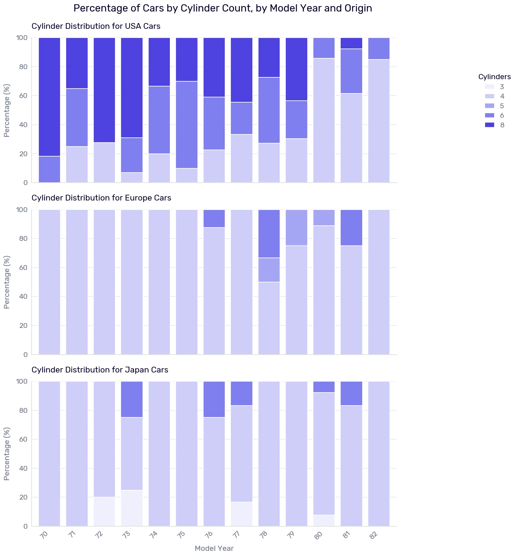
Year by year, this chart is unreadable. The V8 share falls after 1973, but it also falls in 1971, then climbs back in 1976 and 1977. With 15 to 29 American cars a year, a handful of models moves the line several points. Before reading a trend off it, give each number enough cars to mean something.
us = df[df['origin'] == 1].copy()
us['era'] = pd.cut(us['model year'], [69, 73, 79, 82],
                   labels=['70-73', '74-79', '80-82'])
us.groupby('era', observed=True).agg(
    pct_v8=('cylinders', lambda s: round((s == 8).mean() * 100, 1)),
    median_displacement=('displacement', 'median'),
    n=('cylinders', 'size'))
| era | pct_v8 | median_displacement | n |
|---|---|---|---|
| 70-73 | 65.9 | 318 | 88 |
| 74-79 | 37 | 232 | 119 |
| 80-82 | 2.6 | 140 | 38 |
Pooled, the prediction holds: about two thirds of American cars before the crisis were V8s, about a third after, and almost none by 1980.
One caveat before we bank it. The largest single move is 1980, and by then CAFE had been binding for two years and the second oil crisis had happened. The pooled table confirms the fleet shed cylinders across this period. It does not prove October 1973 is why. A prediction that survives rules out the world where nothing happened, not the world where something else did.
What about the miles per gallon? Did the cars get more efficient? More importantly, did the worst (in terms of fuel consumption) cars get more efficient? That could mean a massive shift in consumer behavior or a regulation governing car manufacturing. CAFE again: it passed in 1975 and bound from 1978, so for 1973/1974 only consumer demand and fuel prices should affect the results.
# Calculate the minimum mpg
min_mpg_by_origin_year = df.groupby(['origin', 'model year'])['mpg'].min().unstack(level=0)

fig, ax = plt.subplots(figsize=(10, 6))

for i, (origin_code, origin_name) in enumerate(ORIGIN_NAMES.items()):
    if origin_code in min_mpg_by_origin_year.columns:
        ax.plot(min_mpg_by_origin_year.index,
                min_mpg_by_origin_year[origin_code],
                color=SERIES[i % len(SERIES)],
                marker='o',
                markeredgecolor='white',
                markeredgewidth=1.5,
                label=origin_name)

ax.set_title("Minimum MPG by Model Year and Origin", loc='left')
ax.set_xlabel("Model Year")
ax.set_ylabel("Minimum MPG")
ax.legend(title="Origin", loc="upper left", bbox_to_anchor=(1.02, 1))

plt.tight_layout()
plt.show()
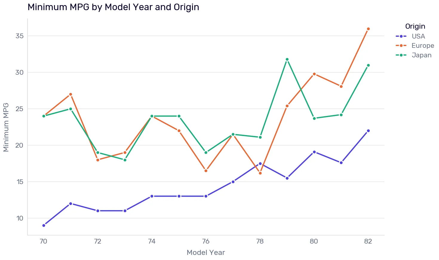
We see a fuel efficiency improvement everywhere in 1974, and growth ever since, but the data looks jagged. How did European cars drop below US cars in 1978? How is the 1980 drop in MPG of Japanese cars even possible?
Let’s check how many values we have for every year and origin region:
sample_counts = df.groupby(['model year', 'origin']).size().unstack(fill_value=0)

fig, ax = plt.subplots(figsize=(10, 6))

for i, (origin_code, origin_name) in enumerate(ORIGIN_NAMES.items()):
    if origin_code in sample_counts.columns:
        ax.scatter(sample_counts.index,
                   sample_counts[origin_code],
                   color=SERIES[i % len(SERIES)],
                   s=50,
                   alpha=0.8,
                   label=origin_name)

ax.set_title("Number of Data Samples per Year by Origin", loc='left')
ax.set_xlabel("Model Year")
ax.set_ylabel("Number of Samples")
ax.legend(title="Origin", loc="upper left", bbox_to_anchor=(1.02, 1))

plt.tight_layout()
plt.show()
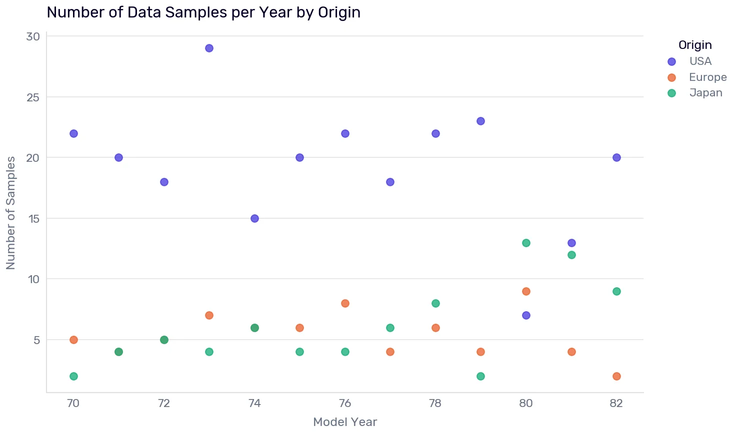
The US cars dominate the dataset. It’s not bad in itself, but other regions have only a handful of values each year (sometimes as few as two values). However, we can at least attempt to explain the 1980 Japanese MPG drop. The dataset simply contains more Japanese cars that year, and the more cars you sample, the more likely one of them is unusually thirsty. After all, we are plotting the minimum, and the more cars you draw, the further down the minimum tends to reach. Nothing changed about Japanese cars in 1980. Something changed about how many of them are in this file. The same arithmetic explains the 1978 European dip: with a handful of cars per year, a single unusual model moves the whole line.
Anything else? We have a dataset of (primarily) passenger cars that, somehow, also contains pickup trucks, for example: International Harvester 1200D and Dodge D200. I would really like to know the thought process behind data sampling/selection, but guess what… nobody documented it.
Is our dataset useless? For any real-world prediction, yes. What about teaching purposes? A bad example is a perfectly valid example. Also, I need flawed data to show you how to deal with those problems. Just remember to be similarly skeptical about your production data.
We spent this chapter distrusting the data. Next chapter, we distrust the model. It will produce a number, that number will be confidently wrong, and the data will be the only thing that tells us why.
-
That is the normal state of documentation, and it is why Rule 1 exists. ↩
-
But that’s classification, not regression, so we won’t do it now. That’s a topic for a later chapter. ↩
-
This problem is called multicollinearity. It doesn’t stop the model from fitting, but it makes the individual coefficients unstable and unsafe to read one at a time. We’ll deal with it later. ↩
-
A backfill is running a data pipeline over historical time periods that it either never covered or covered wrong. ↩
-
Most ML algorithms will fail when we feed them a missing value. Keeping nulls in the dataset is possible, but it limits our options when we choose the algorithm. ↩
-
Honestly, while describing this dataset, I learned more about cars than I ever wanted to know. ↩
-
When you explore production data, pick more data points or find a way to automate the check of all values. ↩
-
Careful: a flat line on its own doesn’t prove the values are net. It’s equally consistent with everything being gross (unlikely, considering the values we have seen in the Automobile Catalog), or with the source recording one horsepower per engine and copying it across years. Again, no way to be sure without proper data lineage and documentation. ↩
-
Except “every model” is doing some work in that sentence. We grouped by the name string, and this file contains “chevroelt chevelle malibu” and “vokswagen rabbit”. A misspelling is a separate group, so any model spelled two ways on either side of 1972 quietly drops out of the table. We also require an exact displacement match, so a model whose engine changed size across the switch drops out too. ↩