
In 2024, a team at Scale AI got suspicious about grade-school math. Language models were scoring near the top of GSM8k, a benchmark of grade-school problems, and nobody could tell whether the models could do arithmetic or had read the answers. GSM8k had been sitting on the public internet for years. So the team wrote a fresh set of problems in the same style, kept them private, and ran the same models again. Several model families dropped by up to 8%. The models most likely to reproduce GSM8k problems word for word were the ones that fell the furthest.1
The drop doesn’t prove the models are useless, and the frontier models of the day held up fine. It shows that a score on data the model has already seen and a score on data it hasn’t are two different measurements, and only the second one tells you anything about tomorrow. The test leaked into the training data, quietly, at a scale where no human could check.
Your model will be wrong. If your predictions come out suspiciously good, something odd happened. Either the answer leaked into the features you trained on, or you scored the model on data it had already seen.2
You can deploy a model that makes mistakes, as long as you can see where it makes them. That depends on whether you built something that could have caught the problems.
Train-test split
Our 392-row CSV has the same problem as the GSM8k dataset. Unlike GSM8k, ours is small enough to inspect row by row.
If we give the model our entire dataset and later test the model using samples from the same dataset (or even the entire dataset), we will measure the performance of the model while working with data it has already seen during the training. We don’t want that. The point of training an ML model is to teach it generalized rules, so it can handle fresh data, something we have never seen before.3
Because of that, we will split the dataset we have into two subdatasets. A part of the data will end up in the training dataset, the one we use to fit the model. The rest will end up in the test dataset. Later, we will compare the test values with the model predictions, and the comparison will tell us how well the model can handle the data it has never seen before.
Every tutorial reaches for the same split: shuffle the rows, put 80% in the training dataset and 20% in the test dataset, fix the random seed so the numbers reproduce tomorrow. Do that here and you get two problems, one of which will make your metric look better than the model is.
from sklearn.model_selection import train_test_split

# Reload from disk, so we don't preserve the variables created during data exploration
df = pd.read_csv(data_url, sep=r"\s+", names=column_names, na_values="?").dropna()

# Separate the independent variables from the target variable
X = df.drop('mpg', axis=1)
y = df['mpg']

# At this point, random_state = 42 is basically a running joke. If you don't know why, read "The Hitchhiker's Guide to the Galaxy"
X_train, X_test, y_train, y_test = train_test_split(X, y, test_size=0.2, random_state=42)
We have the data split. Where is the problem? We have two problems.
During data exploration, we saw years with only two Japanese or European cars. A random split scatters those two rows independently. If both land in test, the model never sees that year-and-region combination while training and has to extrapolate to it. If both land in train, the test set has nothing to say about it. Either way, the metric for that slice is computed from at most one car, and Rule 7 already told you what a statistic from one row is worth. That’s a problem, but that isn’t the worst that happened.
The second problem is data leakage. We know our dataset contains basically identical cars from different years. The values that denote a particular variant (car name and displacement) repeat in multiple rows. If the rest of the columns aren’t an exact match, then the values are nearly identical (there is no meaningful difference between weight 3433 lbs and 3476 lbs).
def model_key(frame):
    return frame['car name'] + " | " + frame['displacement'].astype(int).astype(str)

key_train, key_test = model_key(X_train), model_key(X_test)
shared = sorted(set(key_train) & set(key_test))

pairs = pd.concat([
    pd.concat([
        X_train[key_train == k].assign(mpg=y_train, split='train'),
        X_test[key_test == k].assign(mpg=y_test, split='test'),
    ]).sort_values('model year')
    for k in shared
])
pairs.to_markdown()
We have 15 cars that occur in both the train and test datasets. Start with the worst one.
| cylinders | displacement | horsepower | weight | acceleration | model year | origin | car name | mpg | split | |
|---|---|---|---|---|---|---|---|---|---|---|
| 18 | 4 | 97 | 88 | 2130 | 14.5 | 70 | 3 | datsun pl510 | 27 | test |
| 29 | 4 | 97 | 88 | 2130 | 14.5 | 71 | 3 | datsun pl510 | 27 | train |
Same cylinders, same displacement, same horsepower, same weight, same acceleration, same 27 mpg. One column differs (the model year), and one row landed in train while the other landed in test. We are about to score the model on a row that carries no information the training set didn’t already give it.
The rest are less blatant and no less contaminating. AMC Gremlin 232 occurs three times. AMC Hornet 232 is a totally different car, but you will learn that only by looking at the pictures of it. In our dataset, those two AMC models look the same. And they both have several variants released over the years.
| cylinders | displacement | horsepower | weight | acceleration | model year | origin | car name | mpg | split | |
|---|---|---|---|---|---|---|---|---|---|---|
| 33 | 6 | 232 | 100 | 2634 | 13 | 71 | 1 | amc gremlin | 19 | train |
| 107 | 6 | 232 | 100 | 2789 | 15 | 73 | 1 | amc gremlin | 18 | train |
| 169 | 6 | 232 | 100 | 2914 | 16 | 75 | 1 | amc gremlin | 20 | test |
| 99 | 6 | 232 | 100 | 2945 | 16 | 73 | 1 | amc hornet | 18 | train |
| 127 | 6 | 232 | 100 | 2901 | 16 | 74 | 1 | amc hornet | 19 | train |
| 194 | 6 | 232 | 90 | 3085 | 17.6 | 76 | 1 | amc hornet | 22.5 | test |
df.duplicated().sum() still reports zero. The rows aren’t identical, so nothing flags them, and that silence feels like a passing check. But it’s just another trap. Exact-match deduplication only tells you the rows differ as text. They can still describe the same car. You need business domain knowledge to figure out which columns must match exactly to denote the same thing and which columns allow some slack (while still being the same car).
One more reason to watch out for duplicates or near-duplicates: we have several cars that occur in the same dataset (train) more than once (but they could also reoccur in test, same problem), but have different values of the target variable. What should the model predict in this case?
Near-duplicates with different targets set a practical limit. These rows do differ, in weight, acceleration, and year, so a flexible enough model could separate them. But their feature differences are tiny next to their mpg differences, so any smooth model will split the difference and eat the residual. The hard floor needs feature vectors that are exactly identical with different targets.
Three ways out, and each one costs something. We could go back to data collection and enrich the dataset with a value that helps us distinguish between the cars. We could decide we include only the first/the most recent variant of each car (model + displacement). We may decide we want to use historical data to predict the mileage of cars produced in the future, and use a temporal split instead of a random split.
Let’s split the data based on time (train on years 1970-1979, test on 1980-1982). It will mitigate the problem of having only two data points for some years (now we say: “learn that, for those two years, the values are the same”), and a car that recurs across years is now the thing we predict: next year’s version of a car we already know. However, there is no free lunch in machine learning, so this decision will cause another problem later. Also, this educational dataset wasn’t prepared for being used in this way, so we will get a low-performance model.
train_df = df[df['model year'].between(70, 79)]
test_df = df[df['model year'].between(80, 82)]

X_train = train_df.drop('mpg', axis=1)
y_train = train_df['mpg']

X_test = test_df.drop('mpg', axis=1)
y_test = test_df['mpg']
Training the first model
Now, we train the model. In the first attempt, we take all numeric columns and pass them to the model without thinking about the values and their meaning.
I will explain the linear regression model later. For now, we just run fit():
from sklearn.linear_model import LinearRegression

# Drop 'car name' as this is a text column
X_train_numeric = X_train.drop('car name', axis=1)
X_test_numeric = X_test.drop('car name', axis=1)

model = LinearRegression()
model.fit(X_train_numeric, y_train)
Regression evaluation metrics
predict() will give us numbers. Whether they are any good is a separate question, and scikit-learn offers several ways to answer it (mean_absolute_error, mean_squared_error, r2_score, mean_squared_log_error, median_absolute_error, max_error, and a few others). Each one answers a slightly different question, so let’s look at the math.
In all of the equations below, \(n\) is the number of rows we are scoring, \(y_i\) is the true MPG of row \(i\), and \(\hat{y}_i\) is the MPG the model predicted for that row. Every sum runs over the rows of the dataset being scored, which here is the test set.
Maximum residual error
max_error: the single worst miss in the dataset, in mpg.
Every row except one is ignored, so this reports the worst case rather than the typical one. Not as useless as it looks. It tells us the worst miss we have seen so far, and only so far. The more rows you score, the further the worst miss tends to reach (the same arithmetic that explained the 1980 Japanese MPG drop). Production data will find a worse one, especially if the test dataset doesn’t cover the real-world data well enough.
Our model’s worst miss on the test set: 15.78 mpg.
Mean absolute error (MAE)
mean_absolute_error: the average size of the miss. The good news is that it preserves the units, so if we feed it data in mpg, we get the error value in mpg.
Within one dataset, a single row that is off by 10 mpg contributes as much as 10 rows that are off by 1 mpg each. If we compare two models and one of them makes one huge mistake, while the other many small mistakes, they may both get the same score when we use this metric. Our model’s MAE: 4.23 mpg.
Median absolute error (MedAE)
median_absolute_error: the middle value of the absolute misses instead of their average.
Half of the rows are off by less than this and half by more, and no single row can move it far. The hard part here is explaining the difference between the mean and the median to a manager who heard of the median for the last time 20 years ago. Our model’s MedAE: 3.10 mpg. The mean above the median means a few big misses pull the average up. The histograms below show which ones.
Mean squared error (MSE)
mean_squared_error: the average of the squared misses, in squared units of the target, so in mpg².
Squaring changes the consequences of error size. This metric punishes models that make large errors. One row off by 10 mpg now contributes 100, while the 10 rows off by 1 mpg contribute 10 in total. But squaring the error makes it problematic to use. If your model measures length in meters, you get the error in squared meters. Handy, isn’t it? I dare you to calculate the cost of errors when distance comes out in units of area. MSE still earns its place. It’s the quantity linear regression minimizes while it learns, and it’s a fair way to compare two models scored on the same data. Just don’t put it in a report for people who make decisions.
Our model: about 31 mpg² (5.57 squared). That’s why we have the next metric.
Root mean squared error (RMSE)
root_mean_squared_error: the square root of the mean squared error, which puts the number back into mpg.
The root is taken once, after averaging, not row by row, so the squaring inside still decides how much each row counts. We get the best of two metrics: large errors are punished more, and we still see units we can interpret.
Coefficient of determination (R²)
r2_score, written R²: the model’s squared error divided by the squared error of always predicting the mean of the true values, subtracted from 1.
Here, \(\bar{y}\) is the mean of the true values in the dataset being scored, so the denominator is the spread of those values around their own mean. R² is 1 when every prediction is exact, 0 when the model’s squared error equals that of the mean, and negative when it does worse than the mean. In practice, you will usually see values between 0 and 1, and closer to 1 looks better. R² compares your model with the mean and ignores what its mistakes cost, so a high R² can still hide a model that is worthless where it matters.
Negative R² happens more often than you would expect, and it doesn’t always mean you broke something. It means the model is losing to a flat line drawn through the average of whatever you are scoring. We will see one of those in a minute.
Mean squared logarithmic error (MSLE)
mean_squared_log_error: the mean squared error computed on log-transformed values, which turns differences into ratios.
Predicting 20 mpg for a 10 mpg car counts almost the same as predicting 40 mpg for a 20 mpg car, because both are wrong by the same factor. The \(1 +\) shift keeps a target of zero finite (both values still have to be greater than −1 for the logarithm to exist, which is not a concern for MPG).
Which metric to choose and when a model is good enough?
There is no one right answer. Pick the metric that matches what your mistakes cost:
- One large error costs more than several small ones adding up to the same total: use a metric that squares the error (RMSE).
- Ratios matter more than absolute differences: use the logarithmic error (MSLE).
- Every mpg of error costs the same, regardless of size: use the absolute error (MAE, or MedAE when a few outliers shouldn’t move the number).
- You need a number without units: R² doesn’t change when you convert the target to other units (mpg or km/L gives the same R²), and it tells you how much of the test set’s spread around its own mean the model explains. On a single test set, it ranks models exactly like MSE.
But R² is tied to the rows you score. Two R² values from two different test sets aren’t comparable, because the denominator is the variance of whichever set you happen to be scoring. Our dummy model scores exactly 0 on its own training data and −3.29 on the test set. The same goes for nonlinear transformations of the target: R² computed on log(mpg) and R² computed on mpg answer two different questions. If you train on log(mpg), convert the predictions back to mpg before you score them.
A good number is not enough to earn trust from people who aren’t familiar with machine learning. For a while, I was working at a failing adtech startup. We were building models to predict how much we could pay for an ad slot and still make some money. The models were good, and our ongoing method of manually bidding for ads made our bank account bleed. Still, the CEO was afraid to deploy the models because “what if we bleed out even faster?” Our models beat the baseline of manual bidding every day. We could put the two numbers next to each other. What we couldn’t do was persuade people to trust those numbers.4 Soon, another company purchased the startup to acquire the backend tech, closed all its websites down, and ended the suffering.
To judge a number, we need a baseline and a ceiling. The baseline may be a DummyRegressor (it always predicts the mean value of the training dataset, regardless of input). If our model can’t beat that, we could replace it with the training mean. The ceiling is harder to estimate. Remember the AMC Gremlin and AMC Hornet from the train-test split? Nearly identical features, different MPG. No smooth model can tell rows like that apart, so the MPG spread among such look-alikes is error no smooth model can remove. That noise sets the ceiling.
We could say something like this: “Our regressor gets RMSE 5.57 against a 12.44 baseline (from the dummy model) and against a ceiling limited by the cars that share similar features but differ in MPG.”5 Now, is RMSE 5.57 good? It’s less than half of the baseline’s error, and we haven’t done anything yet to earn it.
And here is the negative R² I promised. Our regressor scores 0.14. The dummy scores −3.29. Nothing broke. The dummy predicts the mean of the training data, 21.08 mpg, while R² grades it against the mean of the data being scored, 31.98 mpg.
Now, compare the two numbers our model got. RMSE says it beats the dummy by more than half. R² says it barely beats a flat line drawn at the test set’s own mean (that line would miss by about 6.0 mpg, and we miss by 5.57). Both are true. Most of our win over the dummy comes from predicting a higher MPG for the 1980s cars overall. We still aim too low (the histograms below show how far), and that bias eats most of what the model gains by telling one car from another.
Our split put the thirsty years on one side of the line and the efficient ones on the other, so the dummy predicts a 1970s average for 1980s cars. A real model can lose the same way. When the test data comes from somewhere the training data has never been, losing to a flat line is a normal result. It doesn’t mean the pipeline is broken.
Debugging regression model errors
A single metric is enough for automated decisions. We could use the metric value to make an automated decision (for example, continuously train new model versions and replace the one in production as soon as you get a better model), but it’s useless when we are asked about the cost of the model’s mistakes. To estimate that, we need more information. For example, a histogram of errors.
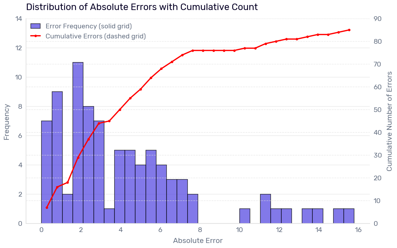
We see that about half of the mistakes made by the model are 3 mpg or less. Of course, we still have room for improvement. Not only the huge mistakes above 10 mpg, but also the cluster between 4 and 8, which constitutes the other half of errors (not counting the extreme ones).
Is this chart informative enough? Partially. We took the absolute errors, so we don’t know whether the model overstates or understates the MPG. We also treat every car equally, and there is a huge difference between a 6 mpg error for a car whose nominal MPG is 10 and for one that goes 30 miles on a single gallon.
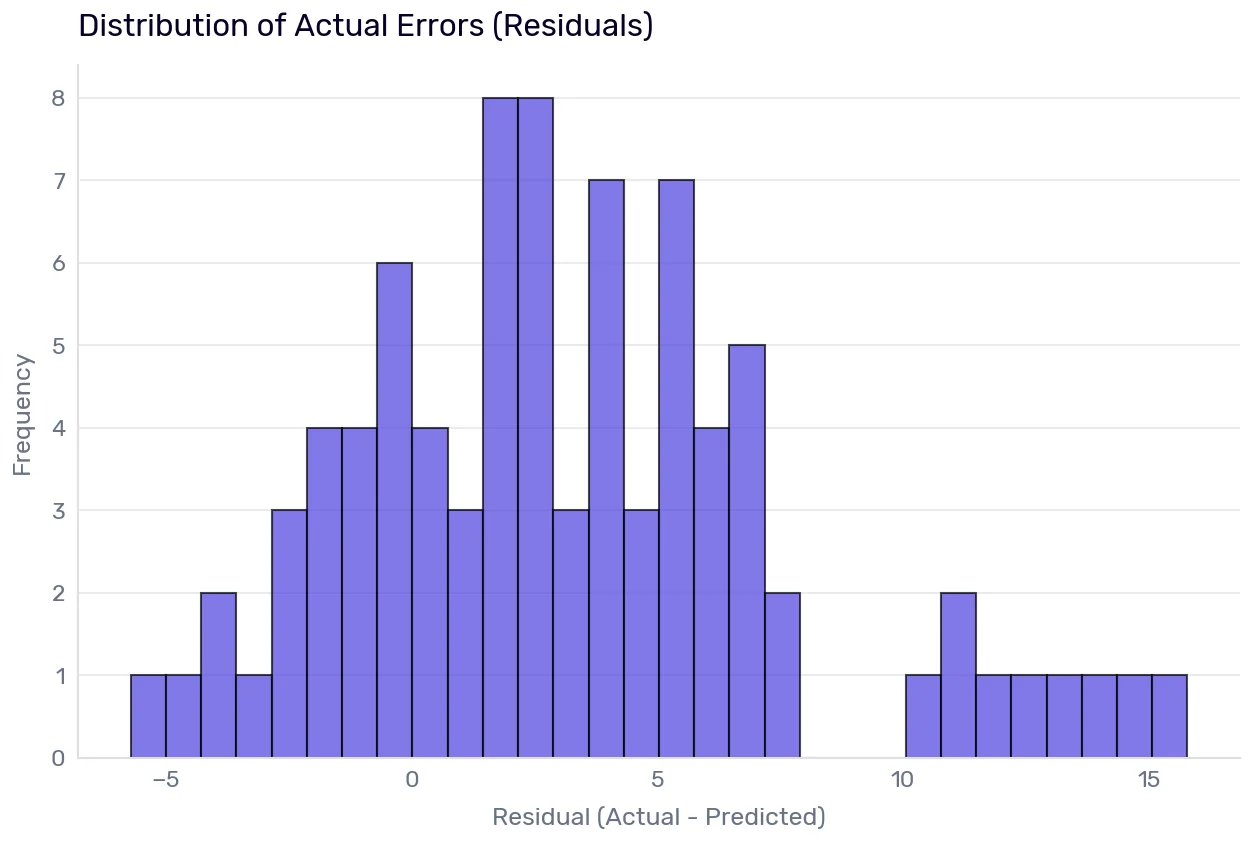
What do we see now? About three in four errors are understatements (the actual value is higher than the predicted one, so actual − predicted gives a number above zero). Our model says the car will go fewer miles on a single gallon than it actually does. Which means that if we used it to budget fuel for a fleet of cars, the fleet would burn less than we planned for. Let’s put a number on it. A car that actually does 30 mpg, predicted at 27 mpg, driving 12,000 miles a year: we budget 444 gallons, and it burns 400. Across 100 such cars, that’s about 4,400 gallons a year sitting in the budget for nothing. Not the worst kind of error (nobody runs out of fuel), but it’s money we could have spent elsewhere. Still, we see only the actual numbers. We have not looked yet at the ratio of errors.
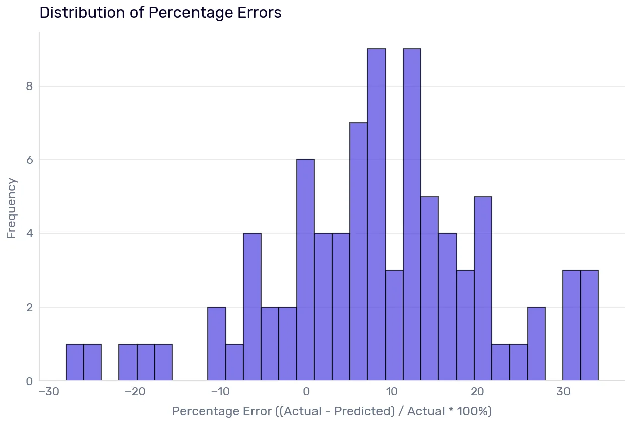
Now, we see that our worst overstatement (actual smaller than predicted, hence a negative value in the chart above), −5.7 mpg, is 28% of that car’s mileage, over on the left. The bars past +30% on the right are a different animal: those are the cars we underestimated by 10 to 16 mpg, missed by a third. The bulk of the distribution sits between 0% and 15%, with the tallest bars around 8% and 13%, which shows the same underestimation on a smaller scale: many cars are around 5-15% better than our model predicts.
Perhaps our very simple model trained on not-preprocessed data cannot grasp the MPG improvement over time (a shocker). However, that’s a problem for the data-preprocessing chapter.
Metrics tell you the model is wrong, and the error distribution tells you how wrong. To find out why, we open the model to see what it learned (feature importance) and go back to the inputs.
Debugging regression model parameters
Dozens of ML explainability tools exist, and you can certainly use one of them, but I want to show you a technique that works regardless of the libraries you use. Pure math. Permutation importance.
However, before we start, let’s clarify why we can’t just look at the model coefficients (model.coef_). Linear model coefficients are the values of a in the linear equation \(\hat{y} = a_1 x_1 + a_2 x_2 + \dots + a_p x_p + b\). It seems that the larger the value is, the more important the feature is. It seems. But that’s not true. We have input values on different scales: units, hundreds, thousands. If the model needs to scale down the weight, the coefficient will be small, but that doesn’t mean the feature isn’t important. Later, we will standardize the input, so comparing coefficients makes more sense.
| feature | coefficient |
|---|---|
| cylinders | -0.487107 |
| displacement | 0.0087759 |
| horsepower | -0.0177635 |
| weight | -0.00541873 |
| acceleration | -0.101063 |
| model year | 0.521265 |
| origin | 0.742794 |
One more thing. What makes a feature unimportant in a linear regression? The neutral element of multiplication is 1, but then we feed the result of multiplication into addition, whose neutral element is 0. Hence, if a column value gets zeroed by the coefficient, it’s not important. But again, if we have to scale down a relatively large (compared to other columns) value, the coefficient applied to an important value that needs scaling down will be indistinguishable from a value reduced to near zero.
Now, the permutation importance. If we don’t dig into the model’s internals and read the coefficients, what do we do instead? First, we score the model normally to get the baseline performance metric. Then, we take each column one by one and randomly shuffle its values. We use the new dataset (with one column shuffled) to score the model again. The drop in the performance metric tells us whether the column is important. If the score doesn’t change, the column isn’t helping the model on the rows we scored: either the model ignores it, or what the model learned about it doesn’t hold on those rows. If we see a large drop, it’s an important column. Hold on to the part about the rows we scored. In a minute, it will matter.
Running the permutation_importance scikit-learn function (permutation_importance(model, X_test_numeric, y_test, n_repeats=30, random_state=42)) on our model against the test dataset tells us that:
| feature | importances_mean | importances_std |
|---|---|---|
| weight | 0.483012 | 0.0951216 |
| origin | 0.0658558 | 0.022379 |
| horsepower | 0.0402631 | 0.00779946 |
| cylinders | 0.0202112 | 0.0117387 |
| model year | -0.0153516 | 0.0100307 |
| displacement | -0.0160963 | 0.0100011 |
| acceleration | -0.0205309 | 0.0067156 |
How to read the table? We didn’t pass a scoring function, so scikit-learn falls back to the model’s own score method. For every scikit-learn regressor, that’s R² (a classifier would give us accuracy instead). The function tests the model several times and calculates R² each time. The importance is the difference between the original R² (without dataset shuffling) and the one after shuffling. We repeat the test 30 times and calculate the mean and standard deviation of the difference. The 0.48 in the weight column means that the model’s R² on average drops by 0.48 when we shuffle the weight column.
The coefficient check showed that weight gets multiplied by −0.005, half a percent of its value and pointing down, but looking at the feature importance, we see it’s the most important feature. How come? Two things. First, a coefficient on its own isn’t comparable with the coefficient next to it, because each one is expressed in the units of its own column. Second, weight’s coefficient is small because it is per pound, and weight runs into the thousands. Multiply the coefficient by how much weight actually varies in the training data (a standard deviation of 881 lbs), and you get a drop of 4.8 mpg. Permutation importance never looks at the coefficient, so the units don’t matter to it. Scaling the data later will change the coefficients but not this table6.
Also, we remember that the origin column looks like a number but isn’t a number. We can’t really interpret its value yet. What else do we see? The top values (if we ignore the origin for now) seem to make sense according to the business-domain rules. Weight, horsepower, and the number of cylinders all affect the mileage of a car.
What do negative values mean? Shockingly, the model does better when we feed it shuffled data for those columns. One thing makes an importance negative, and another makes it small.
The sign comes from the model being wrong about the column on the rows we are scoring. Our model adds 0.52 mpg (look at the coefficient table!) for every model year, which is what the 1970s taught it. On the 1980-1982 cars, the errors run the other way: the later the year, the less the actual mpg exceeds the prediction, and it falls by more per year than the model adds. Shuffling the column partially cancels a slope that no longer holds, and the score improves.
The size comes from how much room the column has to move. Our test set spans only 1980-1982, so a shuffle moves a row by a year or two at most. Whatever the model year contributes across the full 1970-1982 range, shuffling inside three years cannot show it. A narrow range shrinks the importance toward zero from either side, but it cannot push it below zero. Hence the tiny effect (−0.015 R²). Tiny, but larger than its standard deviation across the 30 shuffles. Remember that we split the data by time. This is the first sign of data drift, and it gets its own section.
Displacement and acceleration fail the same test: what the model learned about them doesn’t hold on the 1980s cars. Displacement is the suspicious one: its coefficient is positive, which claims that a bigger engine drives more miles on a gallon. We know that displacement and acceleration are correlated with weight, cylinders, and horsepower. I have not shown you how to verify that yet, but perhaps we see the consequences of multicollinearity here.
Checking and explaining the feature importance reminds me of a story told by my ML professor Tadeusz Morzy. Morzy’s team was building ML models to analyze medical data related to surgeries. At some point, they realized that the amount of blood lost during the surgery is one of the most important features and if a patient lost more than two units7 of blood, they almost always had some post-surgery complications.
The team of IT guys who didn’t know a lot about medicine was proud of itself. The professor said that they even envisioned getting a Nobel Prize in medicine. When they announced the result to the doctors who gave them the data, the doctors started laughing. After that, they showed them the first chapter in a book for medical students. What the team thought to be “groundbreaking results” was literally at the beginning of a “Surgery 101” book.
During the same project, they discovered that when one particular doctor (let’s call him Mr. X) performs a surgery on Monday afternoon, the patient always ends up with some post-surgery problems. The doctors laughed even more and explained that the day of the week doesn’t really matter because Mr. X is a terrible surgeon every day.
Check the feature importance, talk to people who know the domain.
-
Hugh Zhang et al., A Careful Examination of Large Language Model Performance on Grade School Arithmetic, 2024. The fresh benchmark is called GSM1k. The paper reports drops of up to 8% and a correlation between how readily a model reproduces GSM8k problems and how far it falls on the unseen set. It also reports that many models, especially the frontier ones, showed minimal overfitting. ↩
-
If the predictions are exactly right, you are almost certainly using synthetic data generated without noise. Real data never does that. ↩
-
After all, if the production data consisted of only the values we have seen in the past, we could do a database lookup to get the exact value of our target variable. No ML needed. ↩
-
The same problem as trust in self-driving cars (I want to believe it’s the same problem, because it makes my model cooler). Every accident of a self-driving car gets coverage in the news around the world. Thousands of people killed by human-driven cars every day are not even worthy of a footnote. ↩
-
We don’t know yet how many of them we have, because I have not shown you how to cluster similar values. ↩
-
We will scale the values after we deal with the origin column and talk about feature selection, so technically the values will be different. If we only scaled the values and did no other operations, they should stay the same. ↩
-
One “unit of blood” is about 500 ml. ↩