
In the book “How to measure anything” Douglas W. Hubbard uses Monte Carlo simulation to solve the following problem:
Table of Contents
- Probability Distributions
- Fit distribution to data
- How to choose the best distribution using Kolmogorov-Smirnov test
- Monte Carlo simulation
You are considering leasing a machine for some manufacturing process. The one-year lease costs you $400,000, and you cannot cancel early. You wonder whether the annual production level and the savings in maintenance, labor, and raw materials are high enough to justify leasing the machine.
In this article, we are going to implement a Monte Carlo simulation in Python to solve the problem described by D.W. Hubbard.
Probability Distributions
In the problem described in the book, all variables are normally distributed. What should you do if you don’t know what the distribution of your variables is?
I am going to use the Titanic dataset to show you some probability distributions:
RANDOM_STATE = 31415
import matplotlib.pyplot as plt
import numpy as np
import pandas as pd
import seaborn
dataset = seaborn.load_dataset('titanic')
# I want only the age column, but I don't want to deal with missing values
ages = dataset.age.dropna()
Uniform distribution
In the simplest case, all values have the same probability. Let’s generate a uniform distribution of values between 0 and 20 and plot the probability density function.
from scipy.stats import uniform
uniform_dist = uniform(loc = 0, scale = 20)
uniform_dist.rvs(size = 10, random_state = RANDOM_STATE)
x = np.linspace(-5, 25, 100)
_, ax = plt.subplots(1, 1)
ax.plot(x, uniform_dist.pdf(x), 'r-', lw = 2)
plt.title('Uniform distribution of values between 0 and 20')
plt.show()

Bernoulli distribution
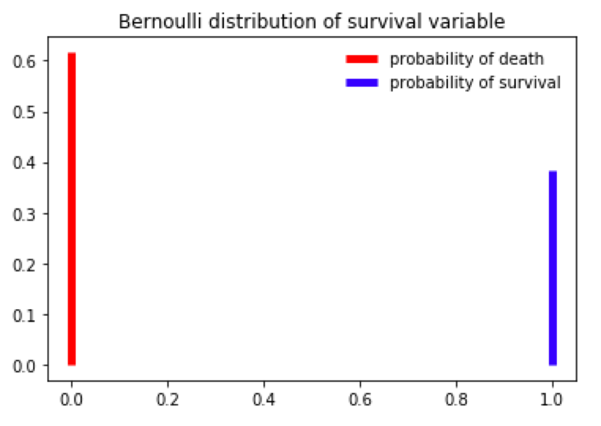
Bernoulli distribution is used when there are only two possible outcomes. I have downloaded the Titanic dataset, so in the next example, I am going to calculate the probability of surviving the accident and plot its chart.
from scipy.stats import bernoulli
countSurvived = dataset[dataset.survived == 1].survived.count()
countAll = dataset.survived.count()
survived_dist = bernoulli(countSurvived / countAll)
# the given value is the probability of outcome 1 (survival) (let's call it p). # The probability of the opposite outcome (0 - death) is 1 - p.
_, ax = plt.subplots(1, 1)
ax.vlines(0, 0, survived_dist.pmf(0), colors='r', linestyles='-', lw=5, label="probability of death")
ax.vlines(1, 0, survived_dist.pmf(1), colors='b', linestyles='-', lw=5, label="probability of survival")
ax.legend(loc='best', frameon=False)
plt.title("Bernoulli distribution of survival variable")
plt.show()
Discrete random variable
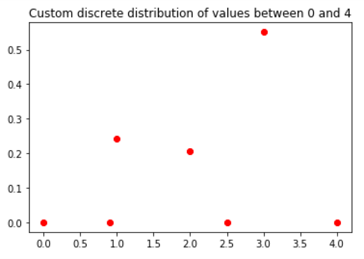
Sometimes we have a discrete variable which has more than two possible states. In this example I will use the pclass variable from the Titanic dataset:
from scipy.stats import rv_discrete
pclass_probability = pd.DataFrame({'probability': dataset.groupby(by = "pclass", as_index=False).size() / dataset.pclass.count()}).reset_index()
values = pclass_probability.pclass
probabilities = pclass_probability.probability
custom_discrete_dist = rv_discrete(values=(values, probabilities))
x = [0, 0.9, 1, 2, 2.5, 3, 4]
_, ax = plt.subplots(1, 1)
ax.plot(x, custom_discrete_dist.pmf(x), 'ro', lw=2)
plt.title('Custom discrete distribution of values between 0 and 4')
plt.show()
Note that only 1, 2, and 3 have a probability higher than 0. Other values did not exist in the given dataset. Hence their probability is 0:
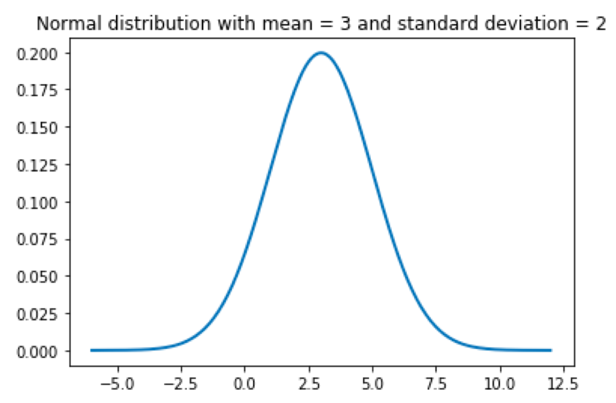
Normal distribution
I guess everyone knows what is going to happen now ;)
from scipy.stats import norm
mean = 3
standard_deviation = 2
normal_distribution = norm(loc = mean, scale = standard_deviation)
x = np.linspace(-6, 12, 200)
_, ax = plt.subplots(1, 1)
ax.plot(x, normal_distribution.pdf(x), '-', lw=2)
plt.title('Normal distribution with mean = 3 and standard deviation = 2')
plt.show()
Gamma distribution
The Gamma distribution looks weird, but it is useful in some circumstances. For example, I could model user behavior on a typical website. The majority of users are going to visit one page and go away. A few are going to click another link and browse a little bit more. Only a handful of them is going to keep clicking and visit more than two pages. In this case, I have to set the loc to 1, to begin the distribution at the point x = 1.
from scipy.stats import gamma
gamma_distribution = gamma(loc = 3, scale = 3, a = 1)
x = np.linspace(0, 12, 200)
_, ax = plt.subplots(1, 1)
ax.plot(x, gamma_distribution.pdf(x), '-', lw=2)
plt.title('Exponential distribution (gamma with a = 1)')
plt.show()

Probability density function or probability mass function?
I use two different functions to calculate probabilities. What is the difference between probability density function (pdf) and probability mass function (pmf)? Probability mass function is used to calculate the probability of discrete values. Probability density function returns the probability of a continuous random variable.
Fit distribution to data
Cool, we can define some distributions, but nobody is going to guess the parameter values to get a distribution that fits their data. So how can we do it automatically?
Fortunately, most distribution implementations in scikit-learn have the “fit” function that gets the data as a parameter and returns the distribution parameters.
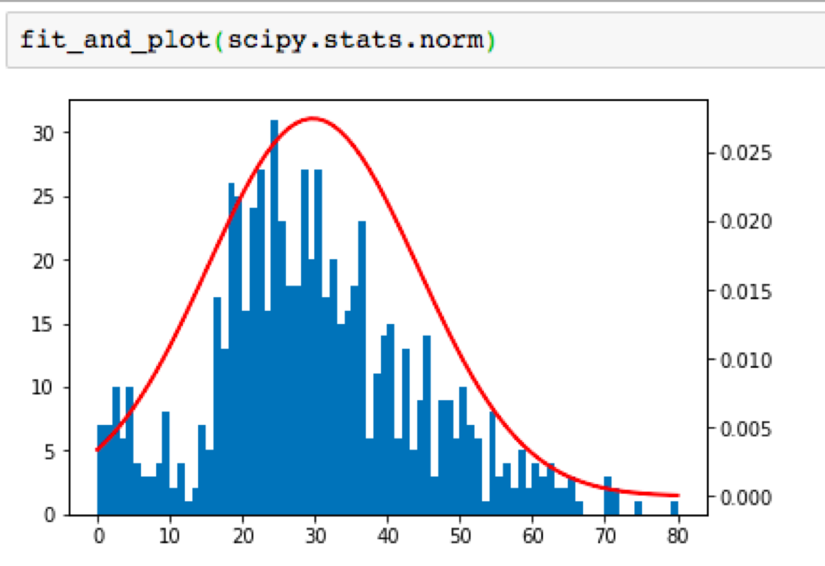
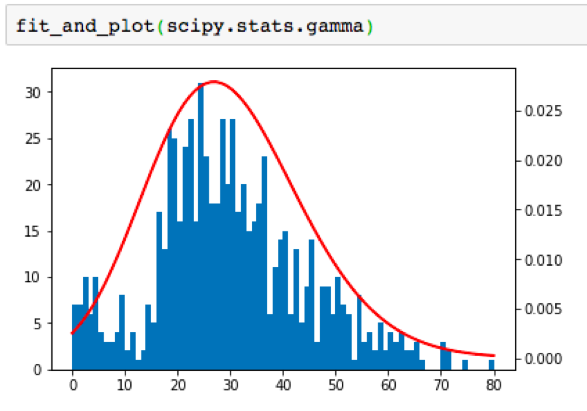
Now it is time to fit the distribution to Titanic passenger age column, display the histogram of the age variable and plot the probability density function of the distribution:
def fit_and_plot(dist):
    params = dist.fit(ages)
    arg = params[:-2]
    loc = params[-2]
    scale = params[-1]
    x = np.linspace(0, 80, 80)
    _, ax = plt.subplots(1, 1)
    plt.hist(ages, bins = 80, range=(0, 80))
    ax2 = ax.twinx()
    ax2.plot(x, dist.pdf(x, loc=loc, scale=scale, *arg), '-', color = "r", lw=2)
    plt.show()
    return dist, loc, scale, arg
Let’s try to fit two distributions:
How to choose the best distribution using Kolmogorov-Smirnov test
According to the definition, the Kolmogorov–Smirnov statistic quantifies a distance between the empirical distribution function of the sample and the cumulative distribution function of the reference distribution.
What does it mean?
It means that we can use this test to verify whether the probability distribution fits the data. In order to do it we must specify the significance level. Usually, 0.05 is used. As in every statistical test if the p-value (calculated by the test) is smaller than the significance level, we reject the null hypothesis.
What is the hypothesis?
Null hypothesis: the data matches the given distribution (there is no difference between both distributions).
Alternative Hypothesis: at least one value does not match the specified distribution (the distributions differ, I use two-sided test, so values are either smaller or greater).
I will use the previously defined function to fit the normal distribution to a given dataset and then perform the Kolmogorov-Smirnov test to check whether it matches the distribution.
from scipy.stats import kstest
dist, log, scale, arg = fit_and_plot(scipy.stats.norm)
d, pvalue = kstest(ages.tolist(), lambda x: dist.cdf(x, loc = loc, scale = scale, *arg), alternative="two-sided")
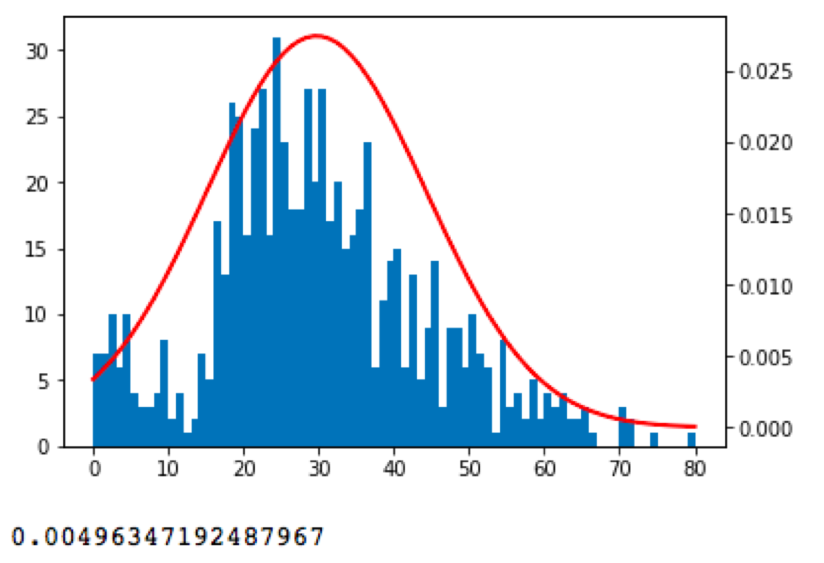
On the chart, we see that the data looks to be normal-ish distributed, but there is a huge difference between actual values and the normal distribution.
That is not the plot we should be looking at. Kolmogorov-Smirnov test calculates the maximal vertical difference between empirical cumulative distributions. Let’s plot the cumulative distributions:
def fit_and_plot_cdf(dist):
    params = dist.fit(ages)
    arg = params[:-2]
    loc = params[-2]
    scale = params[-1]
    x = np.linspace(0, 80, 80)
    _, ax = plt.subplots(1, 1)
    counts, bin_edges = np.histogram(ages, bins=80, normed=True)
    cdf = np.cumsum(counts)
    plt.plot(bin_edges[1:], cdf)
    ax2 = ax.twinx()
    ax2.plot(x, dist.cdf(x, loc=loc, scale=scale, *arg), '-', color = "r", lw=2)
    plt.show()
    return dist, loc, scale, arg
The result looks like this:

Similar, but a little bit weird. As always if p-value is low, the null must go. The p-value is 0.004, so I have to reject the null hypothesis because the given normal distribution does not match the data.
Now I should choose another probability distribution, fit it to the data and perform another test until I finally get one that matches the data. Imagine that I have done it and move to the exciting part ;)
Monte Carlo simulation
What is a Monte Carlo simulation? It is a process that generates a large number of random scenarios based on the input data probability. It calculates what is going to happen when the input is applied to the test function. In the end, the likelihood of results shows which outcome is the most likely.
Finally, we have everything we need to simulate something using the Monte Carlo method. I cannot fit any distribution to Douglas W. Hubbard’s data, because he did not share it, so I have to trust him and just use the value from the book.
The example problem from the How to measure anything book: You are considering leasing a machine for some manufacturing process. The one-year lease costs you $400,000, and you cannot cancel early. You wonder whether the annual production level and the savings in maintenance, labor, and raw materials are high enough to justify leasing the machine.
From your human experts, you got the following ranges of variables (note that all ranges have 90% confidence interval and values are normally distributed):
-
maintenance savings: 10−20 USD per unit
-
labor savings: -2–8 USD per unit
-
raw material savings: 3−9 USD per unit
-
production level: 15,000–35000 units per year
-
annual lease: $400000
-
the annual savings = (maintenance savings + labor savings + raw material savings) * production level
What do the 90% confidence interval and normal distribution mean? Your experts say that they are 90% sure, that the value will be somewhere between the lower and the upper bound. The mean value is the average between the upper bound and the lower bound, so in case of maintenance savings, mean= $15. Standard deviation is defined as (upper bound — lower bound) / 3.29. 3.29 standard deviations equal to 90% of values in normal distribution.
What are we going to calculate? We want to know what is the probability of failure (annual savings smaller than the cost of the machine).
_90_conf_interval = 3.29
maintenance = norm(loc = (20 + 10) / 2, scale = (20 - 10) / _90_conf_interval)
labor = norm(loc = (8 + -2) / 2, scale = (8 - -2) / _90_conf_interval)
raw_material = norm(loc = (9 + 3) / 2, scale = (9 - 3) / _90_conf_interval)
prod_level = norm(loc = (35000 + 15000) / 2, scale = (35000 - 15000) / _90_conf_interval)
number_of_simulations = 1000000
maintenance_results = maintenance.rvs(number_of_simulations)
labor_results = labor.rvs(number_of_simulations)
raw_materials_results = raw_material.rvs(number_of_simulations)
prod_level_results = prod_level.rvs(number_of_simulations)
data = pd.DataFrame({
    "maintenance_savings_per_unit": maintenance_results,
    "labor_savings_per_unit": labor_results,
    "raw_materials_savings_per_unit": raw_materials_results,
    "production_level": prod_level_results
})
data["total_savings"] = (data.maintenance_savings_per_unit + data.labor_savings_per_unit + data.raw_materials_savings_per_unit) * data.production_level
BTW, do you see a mistake? I did not set the random_state parameter of rvs function, so I cannot reproduce my results. Every time I run the code I will get a different outcome!
Speaking of the outcome, we can plot it. I added a vertical line at our profitability threshold:
plt.hist(data.total_savings, bins = 100)
plt.axvline(x = 400000, c = "r")
plt.show()
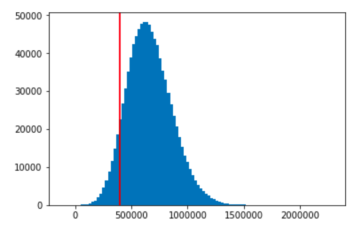
Now, we can count the failures: data[data[“total_savings”] < 400000].count() and easily calculate the probability of annual savings smaller than the cost of the machine (the probability of losing money).
data[data["total_savings"] < 400000].count()["total_savings"] / 1000000
In my case, I got the 0.140153 as the result. Hence the probability of losing money is around 14%.