In this article, I will show you how to use the Savitzky-Golay filter in Python and show you how it works. To understand the Savitzky–Golay filter, you should be familiar with the moving average and linear regression.
Table of Contents
The Savitzky-Golay filter has two parameters: the window size and the degree of the polynomial.
The window size parameter specifies how many data points will be used to fit a polynomial regression function. The second parameter specifies the degree of the fitted polynomial function (if we choose 1 as the polynomial degree, we end up using a linear regression function).
In every window, a new polynomial is fitted, which gives us the effect of smoothing the input dataset.
Take a look at the following animation (Source: Wikipedia Author: Cdang, Licence: CC BY‑SA 3.0)
In every step, the window moves and a different part of the original dataset is used. Then, the local polynomial function is fitted to the data in the window, and a new data point is calculated using the polynomial function. After that, the window moves to the next part of the dataset, and the process repeats.
Python
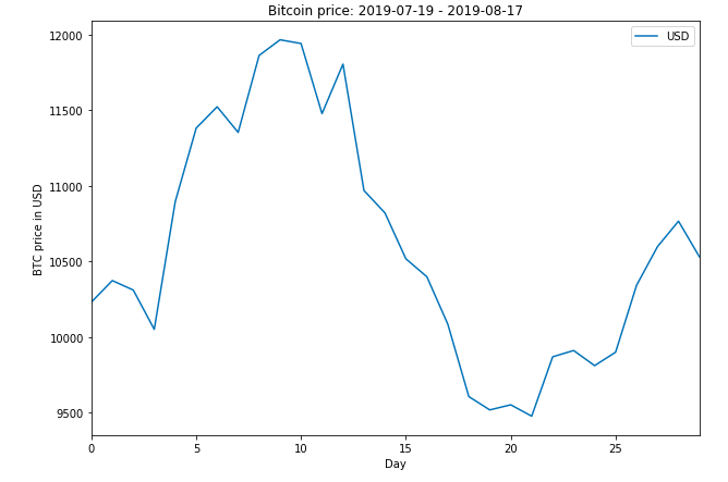
Here is a dataset of Bitcoin prices during the days between 2019-07-19 and 2019-08-17.
bitcoin.plot()
plt.title('Bitcoin price: 2019-07-19 - 2019-08-17')
plt.xlabel('Day')
plt.ylabel('BTC price in USD')
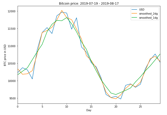
I’m going to smooth the data in 5 days-long windows using a first-degree polynomial and a second-degree polynomial.
from scipy.signal import savgol_filter

smoothed_2dg = savgol_filter(btc, window_length = 5, polyorder = 2)
smoothed_2dg

smoothed_1dg = savgol_filter(btc, window_length = 5, polyorder = 1)
smoothed_1dg

bitcoin['smoothed_2dg'] = smoothed_2dg
bitcoin['smoothed_1dg'] = smoothed_1dg
When we plot the result, we see the original data, and the two smoothed time-series.
bitcoin.plot()
plt.title('Bitcoin price: 2019-07-19 - 2019-08-17')
plt.xlabel('Day')
plt.ylabel('BTC price in USD')