
The last chapter measured how wrong our model is, where, and why. This chapter is about how that measurement becomes wrong without anyone touching the model: the data in production changes, or we reuse the test set until it stops measuring anything.
Data drift
Let’s predict the MPG of a 2019 Skoda Citigo 1.0 MPI (74 hp, displacement: 60.9 cui, 3 cylinders, weight: 1898 lbs, acceleration 0-60 mph: 12.8 s, produced in Europe).
The first problem: how do we pass the model year of something produced after the year 2000? 19? 2019? 119? 79? Because that was the last year in the training dataset?
We encode 1980 as 80. For our model, the timeline starts in 1900, so 2019 is 119 years after the start date. Let’s use 119 as the model year.
When we put that into our model, we get 52.18 mpg. The automobile-catalog site estimates the car’s real-world combined consumption at 38.3 mpg. Off by 14 mpg.
Now, try a 2025 Skoda Scala 1.0 TSI (95) (94 hp, displacement: 60.9 cui, 3 cylinders, weight: 2478 lbs, acceleration 0-60 mph: 10.2 s). Our model predicts 52.07 mpg, the estimate is 37 mpg.1 Off by 15 mpg. A city car and a family hatchback, 580 lbs apart, and the model gives them almost the same number.
The technology changed substantially between 1979 and 2025. Our model may get lucky in some cases, but overall it can’t reliably predict the performance of cars produced 40 years after the ones in the training dataset. Our model is like a Boomer telling Millennials that a single income can support a family.
Checking the inputs
We know the model is wrong about the Scala because we looked up the real value. In production, you don’t get that. You get a prediction, a user who acts on it, and the truth months later, if you ever get it at all. So what can you check on the day the car arrives?
Start with what we already did during data exploration, except the other way around: new data against the training data.
new_cars = pd.DataFrame([
    # 2019 Skoda Citigo 1.0 MPI
    {'cylinders': 3, 'displacement': 60.9, 'horsepower': 74, 'weight': 1898,
     'acceleration': 12.8, 'model year': 119, 'origin': 2},
    # 2025 Skoda Scala 1.0 TSI (95)
    {'cylinders': 3, 'displacement': 60.9, 'horsepower': 94, 'weight': 2478,
     'acceleration': 10.2, 'model year': 125, 'origin': 2},
], index=['citigo', 'scala'])[X_train_numeric.columns]

ranges = X_train_numeric.agg(['min', 'max']).T

for name in new_cars.index:
    ranges[name] = new_cars.loc[name]
    # Does the new value fall between the smallest and the largest value the model was trained on?
    ranges[f'{name} in range'] = new_cars.loc[name].between(ranges['min'], ranges['max'])

ranges.to_markdown()
| min | max | citigo | citigo in range | scala | scala in range | |
|---|---|---|---|---|---|---|
| cylinders | 3 | 8 | 3 | True | 3 | True |
| displacement | 68 | 455 | 60.9 | False | 60.9 | False |
| horsepower | 46 | 230 | 74 | True | 94 | True |
| weight | 1613 | 5140 | 1898 | True | 2478 | True |
| acceleration | 8 | 24.8 | 12.8 | True | 10.2 | True |
| model year | 70 | 79 | 119 | False | 125 | False |
| origin | 1 | 3 | 2 | True | 2 | True |
Two columns fail: the model year and the displacement (a 61-cubic-inch engine is smaller than anything in the training data). Everything else passes.
And that is the whole problem with checking the inputs. Two failed columns out of seven could mean a 1-mpg miss or a 15-mpg miss, and the table looks the same either way. The check can show that an input is outside the training range. It can’t show whether the prediction is wrong.
Checking the distribution
Two cars are too few to measure a distribution. To measure how far data has moved, you need a batch of it, and we have one. The test set is new data as far as the model is concerned, and we split it by time on purpose.
columns = ['mpg', 'cylinders', 'displacement', 'horsepower', 'weight', 'acceleration']

summary = pd.concat([
    train_df[columns].describe().T[['mean', 'std', 'min', 'max']].add_prefix('train '),
    test_df[columns].describe().T[['mean', 'std', 'min', 'max']].add_prefix('test '),
], axis=1)

summary.to_markdown()
| train mean | train std | train min | train max | test mean | test std | test min | test max | |
|---|---|---|---|---|---|---|---|---|
| mpg | 21.0844 | 6.48249 | 9 | 43.1 | 31.9753 | 6.03973 | 17.6 | 46.6 |
| cylinders | 5.78827 | 1.75197 | 3 | 8 | 4.32941 | 0.822138 | 3 | 8 |
| displacement | 213.054 | 108.665 | 68 | 455 | 127.082 | 45.8115 | 70 | 350 |
| horsepower | 111.228 | 40.0894 | 46 | 230 | 80.0588 | 16.4862 | 48 | 132 |
| weight | 3118.63 | 881.504 | 1613 | 5140 | 2468.15 | 438.563 | 1755 | 3725 |
| acceleration | 15.2453 | 2.756 | 8 | 24.8 | 16.6106 | 2.50642 | 11.4 | 24.6 |
fig, axes = plt.subplots(2, 3, figsize=(15, 8))

for ax, column in zip(axes.ravel(), columns):
    bins = np.histogram_bin_edges(df[column], bins=20)
    ax.hist(train_df[column], bins=bins, alpha=0.6, label='train (1970-1979)', density=True)
    ax.hist(test_df[column], bins=bins, alpha=0.6, label='test (1980-1982)', density=True)
    ax.set_title(column)

axes[0][0].legend()
fig.tight_layout()
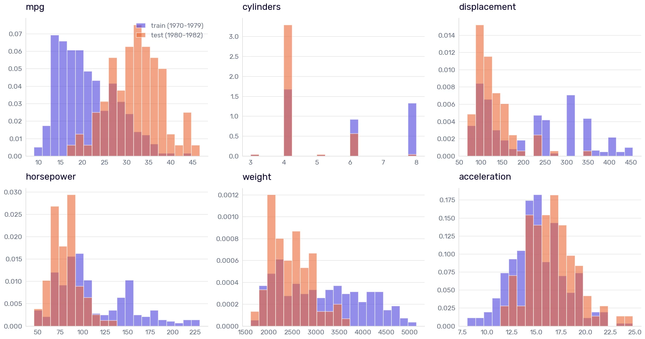
Everything moved. The training data holds a population of big engines between 250 and 450 cui that the test data barely contains, horsepower tops out at 132 instead of 230, the average car loses 650 lbs, and the MPG we are trying to predict goes from 21.08 to 31.98.
The standard deviations moved too, which is easier to miss. Weight goes from 881 to 439, displacement from 109 to 46. The test data also covers a much narrower range.
None of this is our mistake. We chose a temporal split, the second oil crisis hit in 1979, and CAFE fuel-economy targets kept tightening. The inputs moved because the world moved. That has a name: covariate shift, or P(X) moved, where X stands for the input columns.
One warning before we move on. We compared one column at a time, which can only catch a column-by-column move. The Scala weighs 2478 lbs and has a 61-cubic-inch engine. Our training data has plenty of cars at that weight and a few engines that small. Does it have one that combines them? This check will never say.
For that, you have to look at the columns together, which needs standardization and PCA. That picture comes once we learn about both.
Checking the relationship
Back to the strangest number in the feature-importance table: shuffling the model year improved the score. I claimed that the later the year, the less the actual MPG exceeds the prediction. Time to show it.
predictions = model.predict(X_test_numeric)

residuals = pd.DataFrame({
    'model year': X_test_numeric['model year'],
    # Actual minus predicted, so a positive value means the model understated the MPG
    'residual': y_test - predictions,
})

residuals.groupby('model year')['residual'].agg(['mean', 'std', 'count']).to_markdown()
| model year | mean | std | count |
|---|---|---|---|
| 80 | 5.27267 | 5.54451 | 27 |
| 81 | 1.88668 | 3.31621 | 28 |
| 82 | 2.7652 | 3.97529 | 30 |
In 1980, the model understates the MPG by 5.27 mpg. Two years later, it is 2.77. The middle year sits lowest at 1.89, which is not a staircase, and I am not going to pretend it is. With 28 cars and a standard deviation above 3, that gap is noise. What survives is 1980 standing above the other two, and a direction that points down.
np.polyfit(residuals['model year'], residuals['residual'], 1)
# array([ -1.2167003 , 101.86796162])
The residual falls by about 1.2 mpg per model year. Our model adds 0.52 mpg per model year. The error moves against the coefficient and more than twice as fast, which is exactly why shuffling the column improved the score.
Before we call that drift, the objection. The model year is one of our features, and the test set is outside its training range on every single row, because that is what a temporal split does. A straight line asked to continue past the data it was fitted on will drift its residuals by itself, with the world sitting perfectly still.2
That is the Skodas. The model understates the 1980s cars but overstates both Skodas, and the model year explains the flip. The training data ends at 79, and the model adds 0.52 mpg for every year after it. The Citigo is a 119 and collects 21 mpg of optimism nobody ever measured. The Scala is a 125 and collects 24. That’s more than the whole miss.
With both model years pinned at 79, the predictions fall to 31.3 and 28.1 mpg, now 7 and 9 mpg below the estimates. Without the extrapolation, the Skodas look like the 1980s cars: newer than anything the model knows, and more efficient than it expects.
So the first thing to go is the model year. A model fitted without it can’t extrapolate on a column it doesn’t have.
That leaves a second version of the same objection. The 1980s cars are light, and a straight line fitted mostly to heavy 1970s cars will misread light cars too, whatever the calendar says.
Which means we need a control group: light 1970s cars against light 1980s cars. Score the year-blind model on both groups. If being light explains the miss, both groups will miss the same way.
without_year = LinearRegression()
without_year.fit(X_train_numeric.drop('model year', axis=1), y_train)

def mean_residual(X, y):
    return (y - without_year.predict(X.drop('model year', axis=1))).mean()

# Three out of four 1980s cars weigh less than 2800 lbs
light_70s = train_df['weight'] < 2800
light_80s = test_df['weight'] < 2800

train_df.loc[light_70s, 'weight'].mean(), test_df.loc[light_80s, 'weight'].mean()
(np.float64(2254.5846153846155), np.float64(2278.9846153846156))
The 130 light 1970s cars and the 65 light 1980s cars weigh the same on average, within 25 lbs.
mean_residual(X_train_numeric[light_70s], y_train[light_70s]), mean_residual(X_test_numeric[light_80s], y_test[light_80s])
(np.float64(0.4004037469393911), np.float64(6.915987174539122))
On the light 1970s cars, the model is almost unbiased, off by 0.40 mpg.3 On the light 1980s cars, it understates the MPG by 6.92 mpg.
Same model, same average weight, and the model’s average error differs by 6.5 mpg between them. Being light isn’t the problem, because the model reads light 1970s cars correctly. The year can’t be the problem, because the model doesn’t have it. Once the model has accounted for every column it can see, what is left lines up with when the cars were built.
Here is the same thing without any model at all.
fig, ax = plt.subplots(figsize=(10, 6))
ax.scatter(train_df['weight'], train_df['mpg'], alpha=0.6, label='train (1970-1979)')
ax.scatter(test_df['weight'], test_df['mpg'], alpha=0.6, label='test (1980-1982)')
ax.set_xlabel('weight [lbs]')
ax.set_ylabel('mpg')
ax.legend()
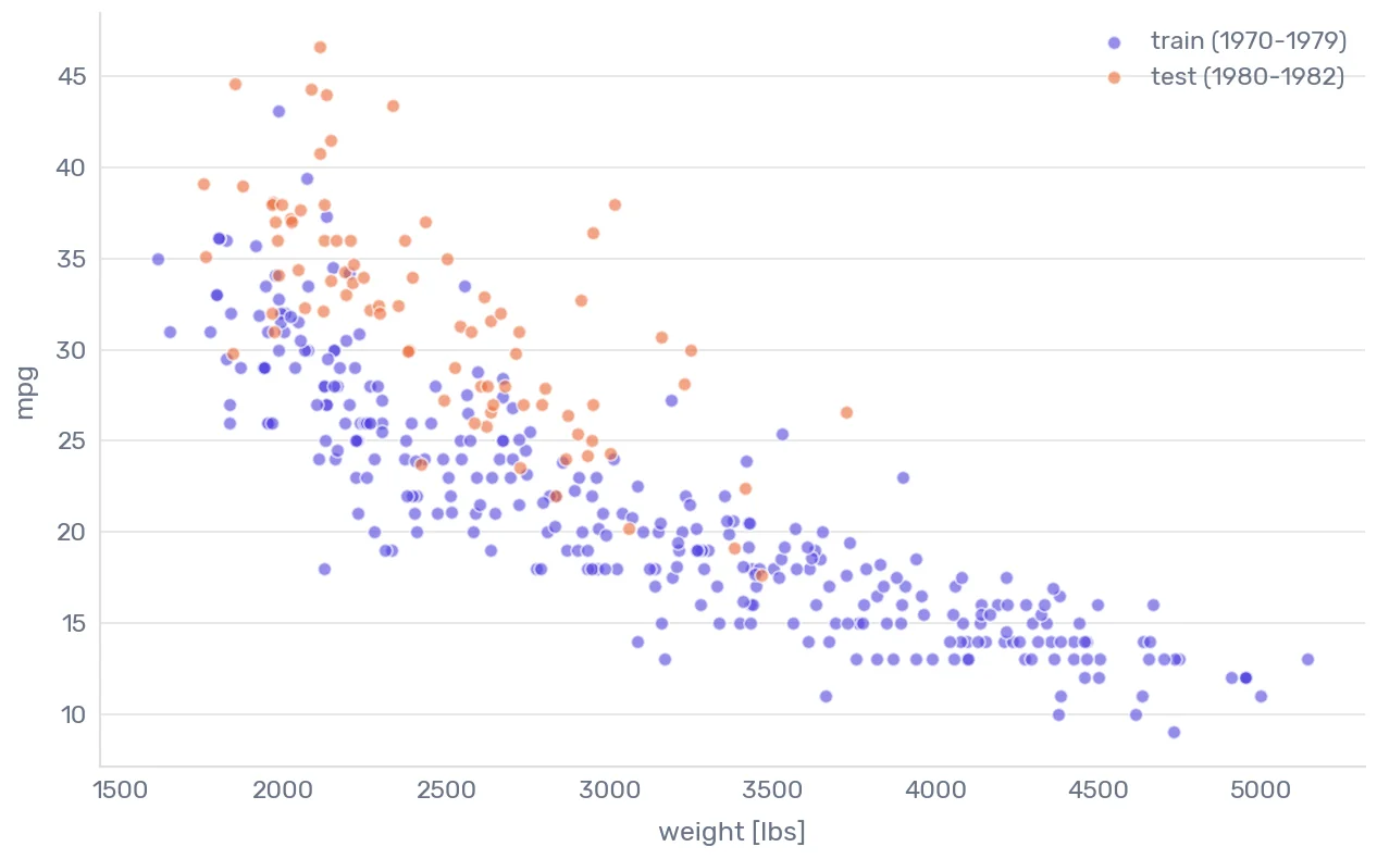
The two clouds overlap between roughly 1,750 and 3,700 lbs, and in that shared band the 1980s cars sit 6 to 10 mpg above the 1970s cars of the same weight. This is concept drift. Covariate shift moves the inputs. Concept drift moves the answer those inputs imply, so a 2,500-pound car in 1981 doesn’t return what a 2,500-pound car returned in 1975, and no column in X changed to warn you. P(y given X) moved.
Now, look at what those checks needed. The residual tables need the true MPG of every test row, and the scatter needs it on the vertical axis. The range check and the histograms never touched the target variable, and no rearrangement of them could have. In production, you don’t have the true MPG on the day you predict.
A deployed model goes stale two ways, and the Skodas manage both at once. Their model year is covariate shift: a value the model has never seen. Without it, what’s left is the concept drift the 1980s cars showed: familiar inputs, a better MPG than the model expects.
Both came from the world moving. The worse kind of concept drift comes from your own model. Users learn what it rewards and change their behavior to collect it.
You can watch it happening in public. Open a certain professional social network and count how many semi-profound business insights arrive illustrated with a vacation photo. Somebody worked out that the length of a reader’s engagement is one of the ranking features. The photo makes you stop. Stopping looks like engagement. The algorithm cannot tell a reader thinking deeply about a post from a reader drooling over a picture.
If you google drift detection in production, you will find a list of statistical tests: Kolmogorov-Smirnov (KS), the population stability index (PSI), the Wasserstein distance, the Jensen-Shannon divergence. Each one is a number for how far two distributions sit apart, doing the job our histograms just did, with a threshold attached so a machine can page somebody at 3 AM.4 Run them on the inputs or on the predictions, and none of them ever sees the true answer. They are cheap and worth having, but none of them can tell you that your users learned to game the model.
For concept drift, you need labels, which means you need to wait, so you need to decide how long you can wait for them. Hold that thought. First, we have a smaller and more embarrassing problem, because I have been scoring this model on the test set over and over for the last few pages.
The danger of overfitting to the test set
Count how many times we have looked at the 1980-1982 cars since we split them off. Every metric in the metrics section. Three error histograms. The permutation importance, shuffled 30 times. The input distributions, the residuals by year, the light-car comparison, and a scatter plot with the true MPG on the vertical axis.
None of those looks changed the model. We fitted it once, before any of them. Apart from the dummy baseline, the only other model we have fitted so far is the year-blind one, and it exists because of what the test set showed us. So does everything we now believe about the model year. That knowledge will shape what we do next, so the test set has already influenced our decisions.
The real damage starts once we begin improving the model. Every change comes with a question: did it help? The tempting answer is to score the test set after every change and keep whatever wins.
The winner’s curse
Take 20 fair coins and flip each one 10 times. The odds are two in three that at least one of them lands heads eight times or more. Crown it the best coin. Flip it 10 more times and expect five.
That coin wasn’t better than the others. We picked it because of a lucky streak.
Scoring models on the test set works the same way. Our test set has 85 cars, and a different 85 cars would give a different RMSE. If you score one model, that noise is harmless: sometimes the number comes out a bit high, sometimes a bit low. If you score 20 and keep the winner, you keep the one the noise flattered. Its test score includes that luck, and the luck won’t repeat in production.
No test car went into fit(). GSM8k leaked through the training data, and this leaks through your decisions, but the score is inflated either way.
Kaggle built its competitions around this problem. Teams submit predictions for a hidden test set, and a public leaderboard scores them on part of it for the whole competition. The final ranking uses the rest, a private leaderboard nobody sees until the end. When it opens, the ranking reshuffles, sometimes by hundreds of places. The community calls it a shake-up.
Train, validation, and test sets
The public leaderboard has a name outside Kaggle: a validation set. The private one is a test set.
So we need three datasets:
- The training set fits the model.
- The validation set chooses between models, features, and settings. Look at it as often as you like, and expect it to flatter you.
- The test set measures the final choice. Once.
“Once” is the part people skip. A test score estimates the performance in production only while nothing you did depended on the test score. Look, change something, and look again, and the second number is a validation score wearing a test set’s name.
Where the validation set comes from
It can’t come from the test set, so it comes out of the training data. We have 307 training cars. If we hold out 60 for validation, we train on 247 cars and choose with a number computed from 60. That’s Rule 7 again: one small group, one noisy number.
Cross-validation stops the waste. Split the training data into K parts, called folds. Train on K − 1 of them and validate on the one left out. Repeat K times and look at all K scores. Every car validates once and trains K − 1 times.
from sklearn.model_selection import cross_val_score

scores = cross_val_score(LinearRegression(), X_train_numeric, y_train, cv=5, scoring='neg_root_mean_squared_error')

# Scikit-learn scorers follow "greater is better", so error metrics come back negated
-scores
array([2.95689235, 2.99595954, 2.46257607, 3.42903564, 3.19680732])
Five folds, five RMSE values, from 2.46 to 3.43. One model, and the verdict moves by almost 1 mpg depending on which cars grade it. Some of that is the coin. Some of it isn’t: the last two folds, the ones that hold the late 1970s, score worst.
Now, what did cv=5 do? For a regression model, it uses KFold(n_splits=5), which cuts the rows into five consecutive blocks and doesn’t shuffle them. Our file is sorted by model year, so each block is two or three model years, and a boundary can fall in the middle of a year.
from sklearn.model_selection import KFold

for _, validation_rows in KFold(n_splits=5).split(X_train_numeric):
    print(sorted(train_df['model year'].iloc[validation_rows].unique()))
[np.int64(70), np.int64(71), np.int64(72)]
[np.int64(72), np.int64(73)]
[np.int64(74), np.int64(75), np.int64(76)]
[np.int64(76), np.int64(77), np.int64(78)]
[np.int64(78), np.int64(79)]
Look at the middle folds. To validate on the mid-1970s, the model trains on the years before them and after them. In production, the model never has data from after the period it predicts.
The obvious fix is worse. KFold(shuffle=True) scatters the years at random, so the Datsun PL510 from 1971 ends up in training while its 1970 twin validates. That’s Rule 8 all over again, this time inside the validation set. A validation set has to follow the same rules as the test set, because it’s asked the same question.
Our question is how a model trained on the past does on the next year. So each fold asks exactly that.5
years = train_df['model year']

# Train on every year before the fold's year, validate on that year
folds = [(np.flatnonzero(years < year), np.flatnonzero(years == year)) for year in range(75, 80)]

scores = cross_val_score(LinearRegression(), X_train_numeric, y_train, cv=folds, scoring='neg_root_mean_squared_error')
pd.Series(-scores, index=range(75, 80)).rename('RMSE').rename_axis('validation year').to_markdown()
| validation year | RMSE |
|---|---|
| 75 | 2.27129 |
| 76 | 2.59498 |
| 77 | 3.16841 |
| 78 | 4.11339 |
| 79 | 3.81283 |
The 1975 fold has the fewest cars to learn from, and it scores best, 2.27. The error climbs to 4.11 on the 1978 cars and eases to 3.81 on 1979. More training data didn’t lower the error.
Look at which cars the model misses in 1978. A Volkswagen Rabbit diesel doing 43.1 mpg, underestimated by 14.7 mpg, in a dataset with no column for fuel type. A Datsun B210 GX, underestimated by 10.5. A Ford Fiesta, by 7.2. Those three and a Mazda GLC are the four 1978 cars in the worst cv=5 fold. Without them, the 1978 RMSE falls from 4.11 to 2.61.
Those cars explain the spike. They don’t explain the direction. For that, freeze a model on 1970-1974 and score it on every later year.
from sklearn.metrics import root_mean_squared_error

early = years <= 74
frozen = LinearRegression().fit(X_train_numeric[early], y_train[early])

for year in range(75, 80):
    later = years == year
    predictions = frozen.predict(X_train_numeric[later])
    # Actual minus predicted, so a positive bias means the model understates the MPG
    bias = (y_train[later] - predictions).mean()
    print(f"{year}: RMSE={root_mean_squared_error(y_train[later], predictions):.2f} bias={bias:+.2f}")
75: RMSE=2.27 bias=+0.33
76: RMSE=2.68 bias=+1.23
77: RMSE=3.80 bias=+2.57
78: RMSE=4.85 bias=+2.53
79: RMSE=5.91 bias=+4.83
The misses lean one way, and they grow. The frozen model understates the MPG by 0.33 mpg in 1975 and by 4.83 mpg in 1979.
Same objection as before: a line fed years it never saw will drift on its own. So rerun the year-by-year folds without the model year. The misses still lean the same way, 0.44 mpg in 1975 and 4.04 mpg in 1979.
The drift from the previous section didn’t start in 1980. And this time, we found it without touching a single 1980s car.
Here is my budget. From here on, every change to the model is judged on the year-by-year folds. The 1980-1982 cars get one look per chapter, after every decision is made. Strictly, that’s more than once, because every look colors the next chapter’s choices. A book has to show you the number. Your project doesn’t: give it one look, at the end.
The last two chapters looked dozens of times. From now on, it’s one look per chapter.
-
Both figures are automobile-catalog’s own estimates of real-world combined consumption, the same method applied to both cars. The official ratings say something else: 54.7 mpg for the Citigo on the European NEDC cycle, and 51.3 mpg for the Scala on WLTP, which replaced NEDC in 2018. Against those, our model looks almost right for both cars, for the wrong reason. The MPG dataset itself was measured on the US city cycle, so no figure here uses exactly the same measuring stick. A change in how the target is measured is drift of its own, and no column in X will warn you about it either. ↩
-
Fuel consumption per mile goes up roughly with weight, and MPG is 1 divided by that, so the true relationship bends. You can see the bend in the scatter plot above. We will straighten it out in the feature engineering chapter. ↩
-
The control cars are part of the training data, so the model has seen them, which flatters that 0.40 a little. A stricter version holds out some 1970s light cars and scores those instead. The gap here is wide enough that it wouldn’t change the verdict. ↩
-
They differ in what they assume. KS works on continuous columns and gets oversensitive on large batches. PSI wants bucketed data and carries folklore thresholds inherited from credit scoring. Wasserstein comes out in the column’s own units, so you have to normalize it before comparing columns. Jensen-Shannon is bounded, which makes it the easiest one to put a threshold on. Pick one, then spend your time on the reference window and the threshold, because those two choices decide what counts as drift. ↩
-
Scikit-learn has a built-in version of this (
TimeSeriesSplit), but likeKFoldabove it cuts by row count, so a fold boundary can land in the middle of a model year. Our rows carry the year, so we cut on the year. ↩