
In Training the first model, I wrote “I will explain the linear regression model later” and went straight to the metrics. Since then, we have called fit() hundreds of times (or, at least, twenty times), built a pipeline around it, and argued about its coefficients for a whole chapter. Then, I kept saying things like “a least-squares fit makes its errors average out to exactly 0” and expected you to take my word for it. This chapter opens the model and checks those claims. I won’t dig into every kind of model, but since I promised you an explanation of the strange terms I used, here it is.
Why look inside the model?
In the case of linear regression, a handful of numbers and one equation are the entire model. Not scikit-learn, not any other library you use, just the math and the values. Once the training is over, all that’s left to do is multiplication and addition, and computers could do both long before anyone wrote a line of Python.
Imagine you have to run the model on an embedded device, like the microcontroller inside a washing machine. You don’t need to buy hardware that can run Python. You train the model in Python and write the equation in C with the coefficients as constants. It runs blazingly fast, without the overhead of an environment capable of running scikit-learn in a washing machine. It’s also much, much cheaper, and somebody has to pay for the extra memory in a million washing machines.
Simple models aren’t useless, either. Remember the tiny neural networks from the model selection step in the machine learning process? Fewer than 500 neurons in total. Those things made real money and kept the company afloat. Simple models have one more advantage. If you ever need to explain the model’s decisions to a regulator, you can understand what happens inside a simple model and describe it to other people. Good luck doing that with a model whose parameters you count in billions.
What is inside the model?
A fitted LinearRegression keeps one number per column in coef_ and one more in intercept_. To predict, it multiplies every column by its number, adds up the products, and adds the constant:
A coefficient (\(a_1\) to \(a_p\)) is the number the model multiplies a column by. It tells you how much the prediction changes when that column grows by one unit and every other column stays where it was. The intercept (\(b\)) is the constant added at the end.
Let’s put our final pipeline in the washing machine. It’s more than the regression, though. The scaler subtracted a mean and divided by a standard deviation it learned, the encoder decided which makes get their own column, and the predictions come out in gallons per 100 miles. If you copy only coef_ and intercept_, the firmware will multiply raw pounds by a number meant for standardized ones, and nothing will crash to tell you.
So we need these numbers too:
regression = final.regressor_
scaler = regression[1].named_transformers_['numeric']

pd.DataFrame({'mean': scaler.mean_, 'standard deviation': scaler.scale_}, index=kept).to_markdown()
| mean | standard deviation | |
|---|---|---|
| horsepower | 111.228 | 40.024 |
| weight | 3118.63 | 880.068 |
| acceleration | 15.2453 | 2.75151 |
pd.concat([
    pd.Series({'intercept': regression[-1].intercept_}),
    pd.Series(regression[-1].coef_, index=regression[1].get_feature_names_out()),
]).to_markdown()
| 0 | |
|---|---|
| intercept | 5.53071 |
| horsepower | 0.922413 |
| weight | 0.738625 |
| acceleration | 0.242859 |
| make_buick | -0.671241 |
| make_chevrolet | -0.157074 |
| make_datsun | -0.643158 |
| make_dodge | -0.482201 |
| make_ford | -0.0223025 |
| make_mercury | -0.13972 |
| make_plymouth | -0.37409 |
| make_pontiac | -1.01458 |
| make_toyota | -0.324366 |
| make_volkswagen | -0.106506 |
| make_infrequent_sklearn | -0.443638 |
The coefficients are in gallons per 100 miles, so a positive one means more fuel. AMC is the make drop='first' removed, and it lives in the intercept. Every rare make, and every make the encoder has never seen, gets the infrequent coefficient.
Here is the whole pipeline in C:
#include <string.h>

static const char *MAKES[] = {
    "buick", "chevrolet", "datsun", "dodge", "ford",
    "mercury", "plymouth", "pontiac", "toyota", "volkswagen",
};
static const double MAKE_COEFFICIENTS[] = {
    -0.671241, -0.157074, -0.643158, -0.482201, -0.0223025,
    -0.13972, -0.37409, -1.01458, -0.324366, -0.106506,
};
static const double INFREQUENT_MAKE = -0.443638;

static const char *MAKE_SPELLINGS[][2] = {
    {"chevy", "chevrolet"}, {"chevroelt", "chevrolet"}, {"maxda", "mazda"},
    {"toyouta", "toyota"}, {"vw", "volkswagen"}, {"mercedes", "mercedes-benz"},
    {"hi", "international harvester"}, {"capri", "mercury"},
};

static const char *add_make(const char *car_name, char *first_word, size_t size) {
    size_t length = strcspn(car_name, " ");
    if (length >= size) {
        length = size - 1;
    }
    memcpy(first_word, car_name, length);
    first_word[length] = '\0';
    for (int i = 0; i < 8; i++) {
        if (strcmp(first_word, MAKE_SPELLINGS[i][0]) == 0) {
            return MAKE_SPELLINGS[i][1];
        }
    }
    return first_word;
}

/* AMC is the dropped make, so its effect lives in the intercept */
static double make_coefficient(const char *make) {
    for (int i = 0; i < 10; i++) {
        if (strcmp(make, MAKES[i]) == 0) {
            return MAKE_COEFFICIENTS[i];
        }
    }
    return strcmp(make, "amc") == 0 ? 0.0 : INFREQUENT_MAKE;
}

double predict_mpg(double horsepower, double weight, double acceleration, const char *car_name) {
    char first_word[32];
    const char *make = add_make(car_name, first_word, sizeof first_word);
    double gallons_per_100_miles = 5.53071
        + 0.922413 * (horsepower - 111.228) / 40.024
        + 0.738625 * (weight - 3118.63) / 880.068
        + 0.242859 * (acceleration - 15.2453) / 2.75151
        + make_coefficient(make);
    return 100.0 / gallons_per_100_miles;
}
For the Skoda Citigo (74 hp, 1898 lbs, 12.8 s, and a make the encoder has never seen), predict_mpg(74, 1898, 12.8, "skoda citigo") comes out at 33.46 mpg, the same as final.predict() in The Skodas in PCA space. No Python, no scikit-learn, and the whole model fits in the memory of a 50-cent microcontroller. Our washing machine predicts the fuel economy of cars. Bear with me.
How does the model learn?
Fitting a model means choosing its parameters (for a linear regression, the coefficients and the intercept) so that the predictions on the training data are as good as possible, where “good” is a measure picked before the training starts.
For LinearRegression, “good” means the smallest sum of squared errors on the training data (ordinary least squares). Your statistics course probably derived the formula: take the derivative, set it to 0, solve the equations. Scikit-learn skips the derivation and hands the columns to SciPy’s least-squares solver (scipy.linalg.lstsq), which returns the coefficients in one step. There’s no training loop, no learning rate, and nothing to babysit while it converges.
If you remember gradient descent from your course, it’s the other way to reach the answer: start somewhere and keep stepping downhill. (Most courses teach gradient descent on a linear regression first, which leaves plenty of people convinced that fit() runs a loop here too. That’s why I’m telling you it doesn’t.) Scikit-learn has it in SGDRegressor, for data too big to solve in one go.
What the fit guarantees
The solution of least squares satisfies this equation, where \(X\) holds the columns plus a column of ones for the intercept:
\[X^\top (y - X\beta) = 0\]\(y - X\beta\) are the errors on the training data. Multiply them by any column, add them up, and you get 0. For the column of ones, that means the errors add up to 0. For every other column, it means the errors have zero correlation with it. Both hold for every least-squares fit with an intercept, no matter how bad the model is.
X = X_train[year_blind]
blind = LinearRegression().fit(X, y_train)
training_errors = y_train - blind.predict(X)
training_errors.mean(), X.corrwith(training_errors).abs().max()
(np.float64(3.7031543231796754e-16), np.float64(3.5496677343381666e-15))
Both are 0, give or take floating-point rounding. It’s also why the reciprocal model in Scoring a transformed target missed its own training cars by 0.25 mpg on average. Its errors added up to 0 in gallons per 100 miles, and we scored them in mpg.
When the answer isn’t unique
If the same column appears twice, any pair of coefficients with the same sum gives the same predictions, and the data has no way to pick one. Scikit-learn doesn’t complain. It returns the pair with the smallest coefficients, so a duplicated weight column gets half of the slope twice. The dummy variable trap is the same problem: three region columns that always add up to the column of ones.
Exact copies are rare. Near copies are all over our data, as the correlation matrix showed. To see what they do, I copied the weight, moved every copied value by about a pound in a random direction, and fitted the model once per fold.
rng = np.random.default_rng(0)
# Every weight again, off by about a pound
almost_twice = X_train[['weight']].assign(weight_again=X_train['weight'] + rng.normal(0, 1, len(X_train)))

coefficients = {}
for (train_rows, _), year in zip(folds, range(75, 80)):
    fitted = LinearRegression().fit(almost_twice.iloc[train_rows], y_train.iloc[train_rows])
    coefficients[year] = pd.Series(fitted.coef_, index=almost_twice.columns)

pd.DataFrame(coefficients).to_markdown()
| 75 | 76 | 77 | 78 | 79 | |
|---|---|---|---|---|---|
| weight | -0.452994 | -0.234364 | -0.104216 | 0.0918197 | -0.0375866 |
| weight_again | 0.447359 | 0.228764 | 0.0984565 | -0.0977508 | 0.0313247 |
The real slope is about −0.0064 mpg per pound. In 1975, the model multiplies weight by −0.45 and its copy by +0.45. In 1978, both flip their signs. Each pair still adds up to roughly the real slope, so the predictions hardly change:
pd.DataFrame({
    'weight once': fold_rmse(LinearRegression(), X_train[['weight']]),
    'weight almost twice': fold_rmse(LinearRegression(), almost_twice),
}).to_markdown()
| validation year | weight once | weight almost twice |
|---|---|---|
| 75 | 2.71615 | 2.88009 |
| 76 | 2.73505 | 2.79396 |
| 77 | 3.45999 | 3.50943 |
| 78 | 4.52069 | 4.54256 |
| 79 | 5.0282 | 5.02994 |
If you only watched the fold scores, you would never notice that the coefficients are garbage.
Reading the coefficients
Interpretability is how well a person can explain why a model made a prediction, in terms they can check against what they know about the problem.
All else equal
Here are the coefficients of each column fitted alone, next to those of the year-blind model with all six:
pd.DataFrame({
    'alone': {column: LinearRegression().fit(X_train[[column]], y_train).coef_[0] for column in year_blind},
    'together': pd.Series(blind.coef_, index=year_blind),
}).to_markdown()
| alone | together | |
|---|---|---|
| cylinders | -2.99787 | -0.224772 |
| displacement | -0.0500235 | 0.000681666 |
| horsepower | -0.12848 | -0.04044 |
| weight | -0.00642702 | -0.00441617 |
| acceleration | 1.00368 | -0.149432 |
| origin | 4.95492 | 0.623622 |
Alone, weight takes the credit for everything that comes with weight: more cylinders, a bigger engine, more horsepower. Together, the other columns take their share, and weight keeps what’s left. Both numbers are correct answers to different questions.
Acceleration is the time from 0 mph to 60 mph in seconds, so a bigger number means a slower car. Alone, each extra second adds 1.00 mpg, because the slow cars are the small, weak ones. Together, at the same weight and horsepower, each extra second takes 0.15 mpg away. Why would a slower car with the same weight and the same horsepower burn more fuel? Gearing, maybe, or automatic transmissions. Neither is in the data, so neither the model nor I can tell you.
“Every other column stays where it was” is also a bit of a fairy tale here. Adding 1,000 lbs to a car without changing its engine or its horsepower describes a car nobody built, and the coefficient answers the question anyway.
What the residuals tell you
Statistics courses list the assumptions behind linear regression: linearity (the relationship is a straight line), independence (the errors don’t depend on each other), equal variance (their spread is the same everywhere), and normality (they follow a normal distribution). You check them by plotting the errors. Here are the year-blind model’s errors on the folds, against what it predicted.
fold_predictions = (y_train[baseline_residuals.index] - baseline_residuals).rename('predicted MPG')

plt.scatter(fold_predictions, baseline_residuals, alpha=0.6)
plt.axhline(0, color='red')
plt.title('Year-blind model: errors on the 1975-1979 folds', loc='left')
plt.xlabel('predicted MPG')
plt.ylabel('actual - predicted [mpg]')
plt.show()
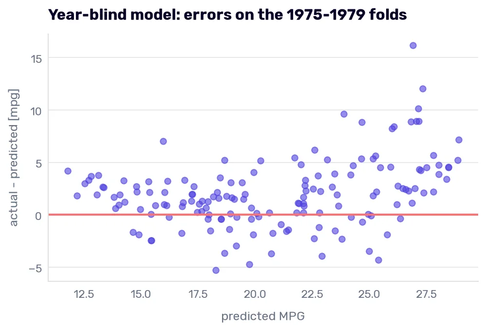
If the assumptions held, you would see a flat band of noise around the red line. Instead, the errors curve up at both ends, three in four of them sit above zero, and the band gets wider toward the right. The curve is the linearity assumption failing. The lean above zero comes from the model year, which this model doesn’t have.
The widening band needs a closer look:
# From the lowest predicted MPG to the highest
QUARTERS = ['lowest 25%', '25-50%', '50-75%', 'highest 25%']
quartiles = pd.qcut(fold_predictions, 4, labels=QUARTERS)
baseline_residuals.groupby(quartiles, observed=True).agg(['mean', 'std', 'count']).to_markdown()
| predicted MPG | mean | std | count |
|---|---|---|---|
| lowest 25% | 1.63054 | 1.9241 | 40 |
| 25-50% | 0.429955 | 2.4048 | 39 |
| 50-75% | 1.7642 | 3.05726 | 39 |
| highest 25% | 4.28123 | 4.03421 | 39 |
The standard deviation of the errors doubles from the gas-guzzlers to the economical cars. Statisticians call unequal spread heteroscedasticity, a word invented to be misspelled. (I knew the problem long before I knew its name. I just googled the term and will forget it by the end of the next paragraph. Skip the name. Just remember that one RMSE hides a 2-mpg spread on some cars and a 4-mpg spread on others.)
Which assumptions matter for prediction?
Linearity, and whatever the lean comes from. Those two put predictions in the wrong place. Independence, equal variance, and normal errors matter for confidence intervals, prediction intervals, and p-values, the tables statistics courses spend weeks on. LinearRegression doesn’t compute any of them (statsmodels does), and this book doesn’t use them. If all you need is predictions, skip the normality test and spend the afternoon on the curve and the lean.
The lean needs information the model doesn’t have, which is Rule 16, and no change to the model will fix it. The curve needs a model that can bend, and that’s what we build in the next chapter, along with the first model in this book that can fit the training data too well.