
The residual plot in Inside the linear regression curved up at both ends, and a straight line can’t follow a curve. So let’s give the model curves. When it works, I’ll be as excited as I was when I bought my first DSLR, and it will end in a similar disappointment. (It turns out a more expensive camera doesn’t turn you into Henri Cartier-Bresson) The surprise is how it fails. I didn’t expect it when I started writing this chapter.
Curves from a linear model
LinearRegression can only add up columns multiplied by coefficients. It can’t bend, but the columns can. PolynomialFeatures makes new columns from the old ones: every square and every product of two columns.
from sklearn.preprocessing import PolynomialFeatures

PolynomialFeatures(2).fit(X_train[['weight', 'horsepower']]).get_feature_names_out()
array(['1', 'weight', 'horsepower', 'weight^2', 'weight horsepower',
       'horsepower^2'], dtype=object)
The column of ones is the intercept, weight and horsepower are the originals, and the other three are new: weight * weight, weight * horsepower, and horsepower * horsepower.
Let’s do it for the columns of the year-blind model. One of them needs fixing first. year_blind still holds origin as a number, and the squares and products would make it worse: Japan squared is 9, Europe squared is 4, and origin × weight multiplies the weight by a region code somebody typed. That’s the numbering problem from One-hot encoding the origin, now inside every product, so the origin gets one-hot encoded before the curves.
I also put a StandardScaler on the numbers, because without it the solver quietly throws information away. The sixth power of 5140 lbs has 23 digits, and LinearRegression treats anything below a millionth of the biggest scale as zero (that’s its tol parameter, which scikit-learn passes to SciPy’s solver since version 1.9, so older versions cut off much less). On the 1975 fold at degree 2, the unscaled columns leave the solver 16 independent directions out of 36 columns. Scaled, it gets 31. At most 32 can exist, because the column of ones repeats the intercept, a 0/1 origin column squared is itself, and nobody is both European and Japanese. The fold takes the last one: every European car before 1975 has 4 cylinders, so origin_Europe cylinders is just a multiple of origin_Europe.
def curved(degree):
    return make_pipeline(
        ColumnTransformer([
            ('numeric', StandardScaler(), numeric),
            ('origin', OneHotEncoder(drop=['USA'], sparse_output=False), ['origin']),
        ], verbose_feature_names_out=False),
        PolynomialFeatures(degree),
        LinearRegression(),
    )

pd.DataFrame({
    'straight': fold_rmse(curved(1), X_named),
    'degree 2': fold_rmse(curved(2), X_named),
}).to_markdown()
| validation year | straight | degree 2 |
|---|---|---|
| 75 | 2.29192 | 2.08871 |
| 76 | 2.81667 | 2.26559 |
| 77 | 3.69986 | 3.42245 |
| 78 | 4.56869 | 4.05081 |
| 79 | 5.07613 | 5.08325 |
From 3.69 to 3.38 on average, and four folds out of five improve. (The straight line scores 3.69 here, not the 3.67 of the year-blind model, because the origin is one-hot encoded now.) That puts the curves level with the whole pipeline from Improving the model (3.33), without the make or the reciprocal target. Here are the fold errors by weight again:
straight_errors = fold_residuals(curved(1), X_named)
curved_errors = fold_residuals(curved(2), X_named)

pd.DataFrame({
    'straight': straight_errors.groupby(bands, observed=True).mean(),
    'degree 2': curved_errors.groupby(bands, observed=True).mean(),
}).to_markdown()
| weight | straight | degree 2 |
|---|---|---|
| (1500, 2200] | 5.49574 | 3.31721 |
| (2200, 2600] | 1.7413 | 1.50951 |
| (2600, 3000] | 0.520124 | 1.28972 |
| (3000, 3500] | 0.46643 | 1.64031 |
| (3500, 4000] | 1.11535 | 2.11307 |
| (4000, 5200] | 2.11727 | 1.75152 |
The error on the lightest cars drops by 2.2 mpg. I didn’t expect the middle to pay for it, but it did: the band from 3000 to 3500 lbs went from 0.47 to 1.64. And every number is still positive. A squared weight column doesn’t know that a 1979 car goes farther on a gallon than a 1975 one.
More curves, worse model
The degree is the highest power PolynomialFeatures goes up to. Degree 2 means squares and products of two columns, degree 3 adds cubes and products of three, and so on. If degree 2 helps, what about degree 3? Or 6?
degrees = {}
for degree in range(1, 7):
    fitted = curved(degree).fit(X_named, y_train)
    degrees[degree] = {
        'columns': fitted[1].n_output_features_,
        'training RMSE': root_mean_squared_error(y_train, fitted.predict(X_named)),
        'fold RMSE': fold_rmse(curved(degree), X_named).mean(),
    }

degrees = pd.DataFrame(degrees).T
degrees.to_markdown()
| columns | training RMSE | fold RMSE | |
|---|---|---|---|
| 1 | 8 | 3.0622 | 3.69065 |
| 2 | 36 | 2.34168 | 3.38216 |
| 3 | 120 | 1.94836 | 8.74426 |
| 4 | 330 | 1.17878 | 70.2551 |
| 5 | 792 | 0.410543 | 242.776 |
| 6 | 1716 | 0.293986 | 405.697 |
plt.plot(degrees.index, degrees['training RMSE'], marker='o', label='training RMSE')
plt.plot(degrees.index, degrees['fold RMSE'], marker='o', label='fold RMSE')
plt.yscale('log')
plt.title('Training and fold errors for every degree', loc='left')
plt.xlabel('polynomial degree')
plt.ylabel('RMSE [mpg], log scale')
plt.legend()
plt.show()
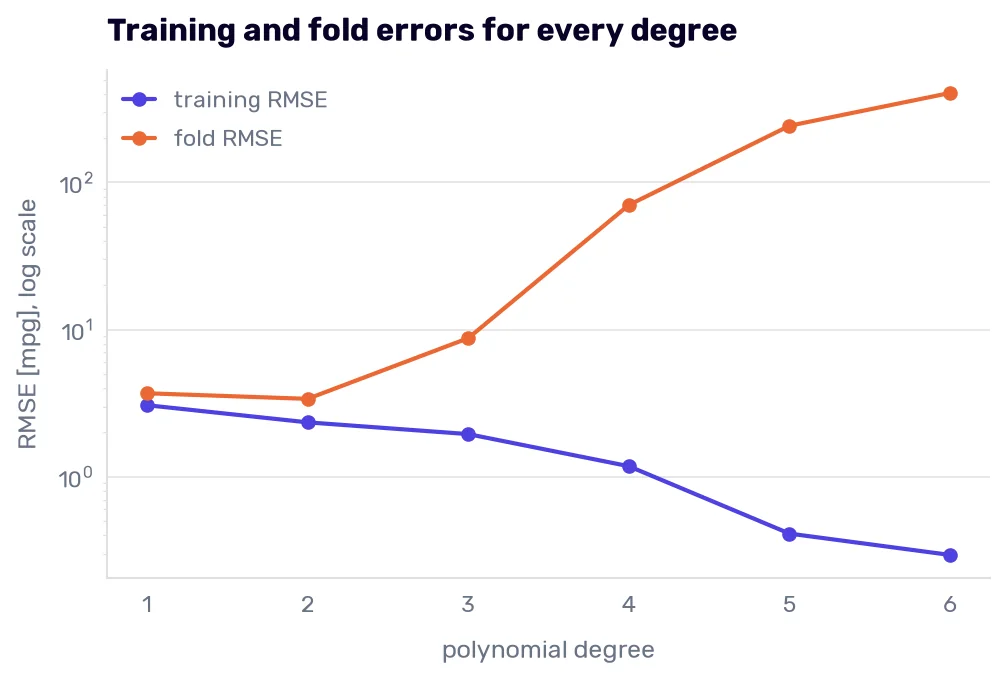
The training error falls with every degree, from 3.06 mpg to 0.29. If I trusted it, degree 6 would be ten times better than anything in this book. On the folds, degree 3 is already more than twice as bad as the straight line, and degree 4 has a fold RMSE of 70 mpg. The y-axis is on a log scale, because otherwise the first three degrees would be a flat line at the bottom.
What we see is called overfitting: the model learns the training rows so well, noise and accidents included, that it gets worse on rows it hasn’t seen. Its opposite is underfitting: a model too simple to follow the pattern, like the straight line that can’t bend. Overfitting shows up as a growing gap between the training error and the validation error. The two columns aren’t measured on the same training cars (the training RMSE comes from a model fitted on all 307, the folds fit on fewer), and on our folds the gap also holds the drift, so at degree 1 most of its 0.6 mpg is the missing year. At degree 4, the gap is 69 mpg.
Statistics has a name for the two ends of that chart, the bias-variance trade-off. Bias is the error you get from a model too stiff to follow the data. The straight line misses the light cars the same way whichever training rows it gets. Variance is the error from a model so flexible that its predictions depend on which rows it happened to see. (Yes, “bias” again. So far, the bias was the lean, the average miss. Here, statisticians mean the misses caused by the model’s shape, like the U in the weight bands. I wish they had picked a second word. And we say that programmers are bad at naming things…)
Why it falls apart
At degree 4, the seven columns (origin is two after one-hot encoding) turn into 330. The 1975 fold trains on the 150 cars from 1970-1974. With more columns than cars, the model can match nearly every training car exactly, and on those 150 cars its RMSE is 0.18 mpg. It has enough coefficients to memorize the list.
That’s the extreme case, though, and you don’t need it to overfit. Degree 3 has 120 columns (fewer than the 150 cars), and its fit on them isn’t perfect (0.94 mpg). It still loses to the straight line on the folds by more than 5 mpg, without ever getting close to memorizing the list.
Here are the worst predictions of degree 4 on the folds, with one more column. In The Skodas in PCA space, we measured how far a car sits from its nearest training car in the five standardized numeric columns. The distance column does the same for every car on the folds, measured against the cars from the years before it.
def nearest_distance(year):
    earlier = X_train['model year'] < year
    scaler = StandardScaler().fit(X_train.loc[earlier, numeric])
    earlier_cars = scaler.transform(X_train.loc[earlier, numeric])
    this_year = X_train[X_train['model year'] == year]
    distances = [np.sqrt(((earlier_cars - car) ** 2).sum(axis=1)).min()
                 for car in scaler.transform(this_year[numeric])]
    return pd.Series(distances, index=this_year.index)

distances = pd.concat([nearest_distance(year) for year in range(75, 80)])
degree_4_errors = fold_residuals(curved(4), X_named)
worst = degree_4_errors.abs().sort_values(ascending=False).head(3).index

pd.DataFrame({
    'car name': X_train.loc[worst, 'car name'],
    'model year': X_train.loc[worst, 'model year'],
    'actual': y_train[worst],
    'predicted': y_train[worst] - degree_4_errors[worst],
    'distance': distances[worst],
}).to_markdown()
| car name | model year | actual | predicted | distance | |
|---|---|---|---|---|---|
| 263 | buick regal sport coupe (turbo) | 78 | 17.7 | 476.861 | 1.39946 |
| 297 | mercedes benz 300d | 79 | 25.4 | -377.061 | 0.90041 |
| 211 | mercedes-benz 280s | 76 | 16.5 | 311.459 | 0.639275 |
A 1978 Buick Regal Sport Coupe with a turbo, predicted at 477 mpg. A car like that would have made the oil crisis somebody else’s problem. And the Mercedes-Benz 300D at −377 mpg makes fuel while driving.
Nothing about those cars is extreme on their own. The Buick’s weight (3445 lbs), horsepower (165 hp), and displacement (231 cui) all sit inside the ranges of the earlier years, so the range check from the data drift section would pass it. The distance doesn’t. At 1.40, the Buick is far from anything built before 1978, and the two Mercedes below it are at 0.90 and 0.64.
The Buick’s model trained on the 242 cars from 1970-1977, with 330 columns. It couldn’t match them all exactly (its training RMSE is 0.85 mpg), but it had enough freedom to need huge coefficients pulling against each other, and a car unlike any of the training cars tips the balance. Is the Buick a one-off?
misses = degree_4_errors.abs()

pd.DataFrame({
    'cars': [(misses > 50).sum(), (misses <= 10).sum()],
    'median distance': [distances[misses > 50].median(), distances[misses <= 10].median()],
}, index=['missed by more than 50 mpg', 'missed by 10 mpg or less']).to_markdown()
| cars | median distance | |
|---|---|---|
| missed by more than 50 mpg | 27 | 0.518894 |
| missed by 10 mpg or less | 100 | 0.207078 |
It isn’t. The cars degree 4 missed by more than 50 mpg (26 of the 27 pass the range check) sit a median 0.52 away from their nearest earlier car, two and a half times farther than the cars it got roughly right. Not every distant car blows up, and not every blowup is distant, but the farther a car is from everything the model trained on, the more room the huge coefficients have to push it around.
Curves in the final pipeline
The curves fixed the light cars without the reciprocal target, so the obvious next step is adding them to the pipeline from Improving the model: PolynomialFeatures on the three kept columns, next to the make and inside the reciprocal target.
def final_with(degree):
    return TransformedTargetRegressor(
        regressor=make_pipeline(
            FunctionTransformer(add_make),
            ColumnTransformer([
                ('numeric', make_pipeline(StandardScaler(), PolynomialFeatures(degree, include_bias=False)), kept),
                ('make', OneHotEncoder(drop='first', min_frequency=10,
                                       handle_unknown='infrequent_if_exist', sparse_output=False), ['make']),
            ], verbose_feature_names_out=False),
            LinearRegression(),
        ),
        func=gallons_per_100_miles,
        inverse_func=gallons_per_100_miles,
    )

pd.Series({degree: fold_rmse(final_with(degree), X_train).mean() for degree in range(1, 5)},
          name='fold RMSE').rename_axis('degree').to_markdown()
| degree | fold RMSE |
|---|---|
| 1 | 3.32873 |
| 2 | 3.46815 |
| 3 | 3.45217 |
| 4 | 4.03048 |
It gets worse. Degree 1 is the final pipeline (3.33), and degree 2 scores 3.47. The pipeline had already dealt with the bend when we switched to gallons per 100 miles, so the extra columns had little left to fix, and their variance cost more than the rest of the bend they fixed.
Both ways of bending land around 3.3 on the folds (3.38 for the curves, 3.33 for the pipeline), and a 0.05-mpg difference between them is noise. I’d pick the reciprocal anyway. I can explain gallons per 100 miles to anyone who has paid for fuel. I can’t explain 36 coefficients on squared standardized columns, and I’d have to if anyone asked why the model predicted what it did.
One look at the test set
Before looking, here is what I expect. Neither the final pipeline nor the degree-2 model has the model year, so both will lose to the first model’s 5.57. That part I’m sure of. Which of the two does better, I’m not. The degree-2 model skips the reciprocal target and its 0.25 mpg of built-in pessimism, but it has 36 columns, and the 1980s cars could bring combinations no training car had. My guess is that they’ll be within half an mpg of each other.
degree_2 = curved(2).fit(X_named, y_train)
X_test_named = X_test.assign(origin=X_test['origin'].map(ORIGIN_NAMES))
test_predictions = {
    'first model': first_model.predict(X_test_numeric),
    'final pipeline': final.predict(X_test),
    'degree 2': degree_2.predict(X_test_named),
}

pd.DataFrame({name: test_metrics(predicted) for name, predicted in test_predictions.items()}).to_markdown()
| first model | final pipeline | degree 2 | |
|---|---|---|---|
| RMSE | 5.56689 | 7.75281 | 7.10136 |
| MAE | 4.2331 | 6.54894 | 5.74747 |
| MedAE | 3.09913 | 6.09326 | 5.16968 |
| max error | 15.7811 | 19.34 | 21.4145 |
| R² | 0.140332 | -0.667336 | -0.398902 |
| mean of actual - predicted | 3.2723 | 6.32258 | 5.6413 |
Both lose to the first model, as expected. My other guess was wrong: the degree-2 model beats the final pipeline by 0.65 mpg of RMSE, more than the half an mpg I allowed. Most of that gap is the last row: the degree-2 model leans 0.68 mpg less. Take the lean away, and the three models look almost the same:
pd.Series({name: (y_test - predicted).std() for name, predicted in test_predictions.items()},
          name='spread of the errors').to_markdown()
| spread of the errors | |
|---|---|
| first model | 4.53033 |
| final pipeline | 4.5134 |
| degree 2 | 4.33895 |
Two tenths of an mpg. The curves don’t know much more about the 1980s cars than the pipeline does. They underestimate them a little less, and the first model still wins because it has the one column the other two don’t.
I’m not switching to degree 2 because of this table. I decided on the pipeline before I looked, and picking the winner now would be the winner’s curse all over again, with the test set as the referee.
Picking a degree by hand is a blunt tool, though. Degree 2 has 36 columns, and nothing stops their coefficients from growing the way degree 4’s did when it sent the Buick to 477 mpg. In the next chapter, we keep the columns and penalize large coefficients instead.