
At the end of Models that don’t draw lines, the tree changed its first question when one more year of cars joined the training data. If one tree is that sensitive to the data it gets, give many trees slightly different data and average their answers. Each tree still misses, but each one misses different cars by different amounts, and averaging the misses cancels some of them out.
Random forest
A random forest trains every tree on a bootstrap sample of the training cars: 307 cars drawn with replacement, so some cars show up two or three times, and about a third don’t show up at all. Nothing stops the trees from growing, so each one memorizes its own sample, and each sample is a little different. The forest predicts the average of all the trees.
The classic recipe also gives every split a random subset of the columns. Scikit-learn’s RandomForestRegressor doesn’t do that by default (max_features=1.0 means every split sees all the columns), so here the bootstrap is the only source of randomness. How many trees do we need?
from sklearn.ensemble import RandomForestRegressor

pd.Series({
    trees: fold_rmse(RandomForestRegressor(n_estimators=trees, random_state=42), X_train[numeric]).mean()
    for trees in [1, 10, 100, 500]
}, name='fold RMSE').rename_axis('trees').to_markdown()
| trees | fold RMSE |
|---|---|
| 1 | 3.28595 |
| 10 | 3.133 |
| 100 | 3.16476 |
| 500 | 3.18275 |
A single fully grown tree on a bootstrap sample scores 3.29. (The fully grown tree in Models that don’t draw lines scored 3.51, so this one drew a lucky sample.) Ten trees bring it to 3.13, and from there, the score settles at about 3.18. The 3.13 was a lucky set of ten samples, and more trees average the luck away. Adding trees doesn’t make a forest overfit. Every new tree is one more vote in the average, so after a few dozen trees, the forest stops changing, and the extra trees only make you wait longer for the result.
The forest gets a free validation set, too. Every tree skipped about a third of the cars, so every car can be scored by the trees that never saw it. That’s the out-of-bag error:
forest = RandomForestRegressor(n_estimators=500, oob_score=True, random_state=42).fit(X_train[numeric], y_train)
out_of_bag = pd.Series(forest.oob_prediction_, index=y_train.index)

pd.Series({
    'training RMSE': root_mean_squared_error(y_train, forest.predict(X_train[numeric])),
    'out-of-bag RMSE': root_mean_squared_error(y_train, out_of_bag),
    'out-of-bag RMSE, per year 1975-1979': np.mean([
        root_mean_squared_error(y_train[X_train['model year'] == year], out_of_bag[X_train['model year'] == year])
        for year in range(75, 80)
    ]),
    'fold RMSE': fold_rmse(forest, X_train[numeric]).mean(),
}, name='RMSE').to_markdown()
| RMSE | |
|---|---|
| training RMSE | 1.01324 |
| out-of-bag RMSE | 2.72675 |
| out-of-bag RMSE, per year 1975-1979 | 2.86507 |
| fold RMSE | 3.18275 |
The training RMSE (1.01) is useless, for the same reason as the 0.12 of the memorizing tree in Models that don’t draw lines: most trees have seen the car they are asked about. The out-of-bag RMSE (2.73) looks like a real validation score, and it costs nothing, but it’s 0.46 mpg more optimistic than the folds. Part of that comes from the cars it scores. It includes the 1970-1974 cars, which the folds never score, so the third row scores only 1975-1979, averaged per year like the folds. That’s still 2.87. The rest of the gap is the year. The bootstrap drew the cars at random, ignoring the year, so a 1978 car is scored by trees that trained on its 1978 neighbors, the same leak as KFold(shuffle=True) in the danger of overfitting to the test set. I’d trust the out-of-bag score on data where next year looks like a random draw from the past years. Our cars get better every year, so I keep using the folds.
Gradient boosting
Gradient boosting builds the trees one after another. It starts from the average MPG of the training cars. The first tree predicts how far each car is from that average. The second predicts what’s still left over, and so on. Each tree is small (three levels by default), and each tree’s correction is multiplied by the learning_rate (0.1 by default) before it’s added, so no single tree can move a prediction far.
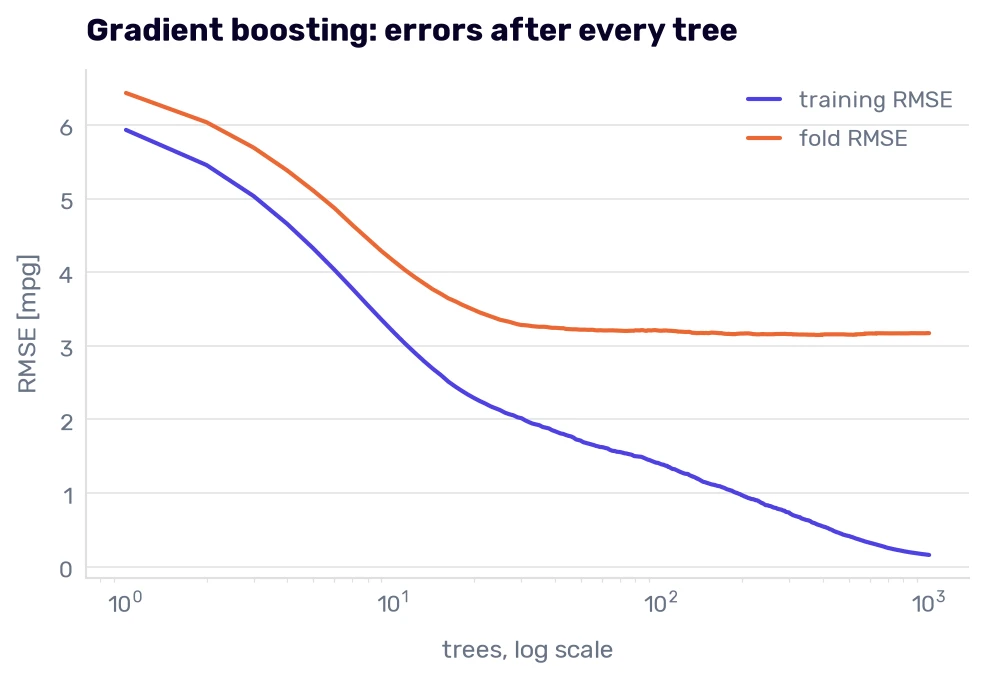
The forest averages trees that don’t know about each other. Boosting adds trees where each one fixes the previous ones, which means it can keep fixing the noise in the training data too. staged_predict() returns the prediction after every tree, so we can watch it happen:
from sklearn.ensemble import GradientBoostingRegressor

boosting = GradientBoostingRegressor(n_estimators=1000, learning_rate=0.1, max_depth=3, random_state=42)

fold_curves = {}
for year, (train_rows, validation_rows) in zip(range(75, 80), folds):
    fitted = clone(boosting).fit(X_train[numeric].iloc[train_rows], y_train.iloc[train_rows])
    fold_curves[year] = [root_mean_squared_error(y_train.iloc[validation_rows], predicted)
                         for predicted in fitted.staged_predict(X_train[numeric].iloc[validation_rows])]

fitted = clone(boosting).fit(X_train[numeric], y_train)
curves = pd.DataFrame({
    'training RMSE': [root_mean_squared_error(y_train, predicted) for predicted in fitted.staged_predict(X_train[numeric])],
    'fold RMSE': pd.DataFrame(fold_curves).mean(axis=1).to_numpy(),
}, index=range(1, 1001))

plt.plot(curves.index, curves['training RMSE'], label='training RMSE')
plt.plot(curves.index, curves['fold RMSE'], label='fold RMSE')
plt.xscale('log')
plt.title('Gradient boosting: errors after every tree', loc='left')
plt.xlabel('trees, log scale')
plt.ylabel('RMSE [mpg]')
plt.legend()
plt.show()
curves.loc[[1, 10, 50, 100, curves['fold RMSE'].idxmin(), 1000]].rename_axis('trees').to_markdown()
| trees | training RMSE | fold RMSE |
|---|---|---|
| 1 | 5.93172 | 6.43365 |
| 10 | 3.18443 | 4.15148 |
| 50 | 1.71118 | 3.21915 |
| 100 | 1.38982 | 3.20453 |
| 384 | 0.571142 | 3.1458 |
| 1000 | 0.159228 | 3.17177 |
After one tree, both errors sit around 6 mpg, close to the 6.48 standard deviation of the training MPG, because one tree moves every prediction only a tenth of the way from the average. By 50 trees, the fold error is down to 3.22, and from there it barely moves: 3.15 at its best (384 trees) and 3.17 at 1000. The training error keeps falling the whole way, to 0.16. It’s the same gap as in Bending the line (Rule 18), but where the degree-4 curves blew up, boosting overfits so slowly that the 616 trees after the best one cost us 0.03 mpg.
GradientBoostingRegressor is the textbook version. Scikit-learn’s HistGradientBoostingRegressor does the same thing faster: it sorts every column into at most 255 bins before looking for splits, so it tries 255 thresholds per column instead of every value. On 307 cars, speed doesn’t matter, but on a few million rows it’s the difference between minutes and hours. (Or, as every AI startup in 2024 and 2025 would say: “Train it in minutes, not hours.”) Its defaults grow different trees, though: up to 31 leaves with at least 20 cars each, instead of three levels. (The min_samples_leaf from the previous chapter, again.) You will also meet XGBoost, LightGBM, and CatBoost, which are separate libraries built on the same idea, with more settings and more speed. I use them on large tables. On 307 cars, scikit-learn’s version is enough.
Here are the forest and the boosting model (with its defaults, 100 trees) next to the final pipeline:
from sklearn.ensemble import HistGradientBoostingRegressor

hist_boosting = HistGradientBoostingRegressor(random_state=42)

pd.DataFrame({
    'forest': fold_rmse(forest, X_train[numeric]),
    'boosting': fold_rmse(hist_boosting, X_train[numeric]),
    'final pipeline': fold_rmse(final, X_train),
}).to_markdown()
| validation year | forest | boosting | final pipeline |
|---|---|---|---|
| 75 | 2.3516 | 2.20807 | 2.28193 |
| 76 | 2.32483 | 2.34285 | 2.71561 |
| 77 | 2.58476 | 2.34068 | 3.09116 |
| 78 | 3.82752 | 3.56099 | 4.18162 |
| 79 | 4.82505 | 4.96651 | 4.37335 |
Boosting averages 3.08, the best year-blind number in this book. It wins 1975-1978 by 0.07 to 0.75 mpg and loses 1979 by 0.59. The forest (3.18) wins three years and loses 1975 and 1979. The tuned Ridge and the nearest neighbors had the same shape: a lead that changes more from one year to the next than its average size, and a loss in the year closest to the cars we have to predict. Under Rule 19, both are ties with the pipeline. (I hoped one of them would finally win 1979. None of the models that replaced the line has.)
Which columns do the trees use?
A forest has no coefficients to read, but it has an attribute called feature_importances_. Every split lowers the squared error of the training cars it divides, and the attribute adds up those drops per column, over all splits in all trees, scaled to sum to 1:
pd.Series(forest.feature_importances_, index=numeric, name='impurity importance').sort_values(ascending=False).to_markdown()
| impurity importance | |
|---|---|
| weight | 0.596702 |
| cylinders | 0.156762 |
| horsepower | 0.10822 |
| displacement | 0.0900075 |
| acceleration | 0.0483078 |
Weight first, which we expected, and cylinders second, ahead of horsepower and displacement. Before you trust that, remember what it measures: how much each column helped split the training cars. A tree that memorizes the training data gets credit for every split it made while memorizing. And when two columns carry the same information, the credit goes to whichever one the tree happened to split on first.
Choosing what to keep measured importance the other way, by shuffling a column on the validation years and watching the RMSE grow. Here is the same measurement for the forest:
importances = {}
for (train_rows, validation_rows), year in zip(folds, range(75, 80)):
    fitted = clone(forest).fit(X_train[numeric].iloc[train_rows], y_train.iloc[train_rows])
    result = permutation_importance(
        fitted, X_train[numeric].iloc[validation_rows], y_train.iloc[validation_rows],
        scoring='neg_root_mean_squared_error', n_repeats=30, random_state=42,
    )
    importances[year] = pd.Series(result.importances_mean, index=numeric)

importances = pd.DataFrame(importances)
importances['mean'] = importances.mean(axis=1)
importances.sort_values('mean', ascending=False).to_markdown()
| 75 | 76 | 77 | 78 | 79 | mean | |
|---|---|---|---|---|---|---|
| weight | 1.35684 | 2.08554 | 3.34075 | 3.184 | 2.66186 | 2.5258 |
| displacement | 1.54884 | 2.38076 | 1.57645 | 0.855274 | 0.405773 | 1.35342 |
| acceleration | 0.169238 | 0.214904 | 0.237652 | 0.02124 | 0.0567029 | 0.139947 |
| cylinders | 0.0102275 | 0.0158068 | 0.0560771 | 0.0379977 | 0.266962 | 0.0774143 |
| horsepower | -0.08561 | 0.164419 | 0.121899 | -0.0235239 | 0.129006 | 0.0612378 |
On cars it hasn’t seen, the forest needs weight (2.53 mpg) and displacement (1.35). Cylinders, second by the built-in importance, add 0.08. Horsepower adds 0.06, less than acceleration.
Compare that with the linear model. In Choosing what to keep, we dropped displacement and kept horsepower, and horsepower was the second most important column. The forest went the other way, and I can’t call either choice wrong. Weight, displacement, horsepower, and cylinders are near copies of each other, and each model picked its own representative from the block, the way the coefficients traded their effects under Rule 15. So when someone asks me which column matters, I ask which model they mean. Before you believe any of these tables, check them against what you know about cars (Rule 12).
The year comes back
In Dropping the model year, we dropped the year even though it improved every fold. The reason was the Skodas. A straight line keeps adding 0.52 mpg per year, and a 2019 car sits 40 years past the end of the data, so the first model gave the Skodas 52 mpg.
A tree can’t do that. A split on the year asks something like “model year <= 76.5”, and a 2019 car answers it the same way a 1979 car does. Everything past the last training year lands in the same boxes as 1979. Every tree is flat beyond its last threshold, so a forest that averages trees and a boosting model that adds them up are flat there too. (Boosting isn’t held under the ceiling from Rule 20, because a sum of corrections can go past the best training MPG, but it can’t keep climbing with the year.) So the reason we dropped the year doesn’t apply to trees. Let’s put it back:
with_year = numeric + ['model year']

pd.DataFrame({
    'first model': fold_rmse(LinearRegression(), X_train_numeric),
    'forest, with year': fold_rmse(forest, X_train[with_year]),
    'boosting, with year': fold_rmse(hist_boosting, X_train[with_year]),
    'final pipeline': fold_rmse(final, X_train),
}).to_markdown()
| validation year | first model | forest, with year | boosting, with year | final pipeline |
|---|---|---|---|---|
| 75 | 2.27129 | 2.21298 | 1.91362 | 2.28193 |
| 76 | 2.59498 | 2.19838 | 2.20905 | 2.71561 |
| 77 | 3.16841 | 2.2017 | 2.06428 | 3.09116 |
| 78 | 4.11339 | 3.35691 | 3.05092 | 4.18162 |
| 79 | 3.81283 | 3.88615 | 3.73194 | 4.37335 |
Boosting with the year averages 2.59. It beats the final pipeline in every year, by 0.37 to 1.13 mpg, and the lead never changes from one year to the next by more than its average size (0.73), so Rule 19 lets it count. Against the first model, boosting wins every year too, but its lead falls from 1.06 in 1978 to 0.08 in 1979, a drop of more than its average of 0.60, so Rule 19 calls that one a tie. The first model is still out because of the Skodas.
And the Skodas?
boosting_with_year = clone(hist_boosting).fit(X_train[with_year], y_train)
boosting_with_year.predict(new_cars[with_year])
array([33.28472612, 27.51319685])
The boosting model predicts 33.28 and 27.51 mpg, against real-world estimates of 38.3 and 37. That’s about what the final pipeline predicted (33.46 and 26.98), and nowhere near the first model’s 52 mpg. Boosting treats both Skodas as 1979 cars, which is what we did to the line by hand in the data drift section when we pinned their year at 79 (31.3 and 28.1 mpg). The trees do it to every car past 1979 without being told.
One look at the test set
Rule 14 says to decide in advance how many looks you get. This is the last chapter about regression, so it gets the one look I planned for the end: the best model of each kind on the 1980-1982 cars. The first model and the final pipeline we have scored already (5.57 and 7.75). The two new ones are the forest and the boosting model, both with the year.
Before looking, here is what I expect. Both tree models know that a 1979 car does better than a 1975 car with the same specs, which the pipeline doesn’t, so both should beat its 7.75. But to a tree, every 1980s car is a 1979 car. The first model keeps adding 0.52 mpg per year past the end of the data, and from 1980 to 1982 that trend was still running. So I expect both tree models to land between the two linear ones, around 6.5, with boosting ahead of the forest by about as much as on the folds. If either of them beats 5.57, the folds were right about the trees, and I was wrong about the trend.
I’m shipping boosting with the year, because it won the folds. This table only measures it.
forest_with_year = clone(forest).fit(X_train[with_year], y_train)
test_predictions = {
    'first model': first_model.predict(X_test_numeric),
    'final pipeline': final.predict(X_test),
    'forest, with year': forest_with_year.predict(X_test[with_year]),
    'boosting, with year': boosting_with_year.predict(X_test[with_year]),
}

pd.DataFrame({name: test_metrics(predicted) for name, predicted in test_predictions.items()}).to_markdown()
| first model | final pipeline | forest, with year | boosting, with year | |
|---|---|---|---|---|
| RMSE | 5.56689 | 7.75281 | 4.95584 | 4.99702 |
| MAE | 4.2331 | 6.54894 | 3.75798 | 3.72294 |
| MedAE | 3.09913 | 6.09326 | 3.36 | 3.1566 |
| max error | 15.7811 | 19.34 | 17.9732 | 17.2297 |
| R² | 0.140332 | -0.667336 | 0.318699 | 0.307329 |
| mean of actual - predicted | 3.2723 | 6.32258 | 2.90853 | 2.6708 |
Both tree models beat the first model, with an RMSE of 4.96 for the forest and 5.00 for boosting, against 5.57. My guess of “around 6.5” was wrong, and so was the reasoning behind it. The first model’s 0.52 mpg per year was supposed to give it the edge on the 1980s cars, and it still leans more (3.27 mpg) than either tree model (2.91 and 2.67). My best guess is the curve in weight that we found in the bend in the residuals. There, the year-blind straight line understated the lightest cars by 5.29 mpg against 0.26 in the middle, three in four 1980s cars weigh under 2800 lbs, and a tree can follow the bend. Checking would mean digging through the test cars, so it stays a guess (Rule 14). The forest’s RMSE is 0.04 lower than the boosting model’s. Boosting has the lower MAE, median error, and lean.
pd.Series({name: (y_test - predicted).std() for name, predicted in test_predictions.items()},
          name='spread of the errors').to_markdown()
| spread of the errors | |
|---|---|
| first model | 4.53033 |
| final pipeline | 4.5134 |
| forest, with year | 4.0364 |
| boosting, with year | 4.24845 |
Take the lean away, as in Bending the line, and the spread drops from 4.53 for the first model to 4.25 for boosting and 4.04 for the forest. The degree-2 curves got 0.19 off it. Boosting does a little better than that, and the forest does more than twice as well, which is where its lower RMSE comes from.
Look at the last row, though. Every model in this table still predicts the 1980s cars too low, by 2.7 mpg at best. Here are the boosting model’s worst misses:
boosting_predictions = test_predictions['boosting, with year']
pd.DataFrame({
    'car name': X_test['car name'], 'actual': y_test, 'predicted': boosting_predictions,
    'residual': y_test - boosting_predictions,
}).sort_values('residual', ascending=False).head(6).to_markdown()
| car name | actual | predicted | residual | |
|---|---|---|---|---|
| 387 | oldsmobile cutlass ciera (diesel) | 38 | 20.7703 | 17.2297 |
| 322 | mazda glc | 46.6 | 33.8868 | 12.7132 |
| 333 | datsun 280-zx | 32.7 | 20.1981 | 12.5019 |
| 326 | vw dasher (diesel) | 43.4 | 31.6622 | 11.7378 |
| 394 | vw pickup | 44 | 33.0867 | 10.9133 |
| 327 | audi 5000s (diesel) | 36.4 | 25.5092 | 10.8908 |
Three names say diesel, and the Volkswagen pickup at 44 mpg is almost certainly a fourth: its 97-cubic-inch, 52-horsepower engine matches VW’s 1.6-liter diesel, and the gasoline engine VW put in that pickup made over 70 hp. Then there’s a Mazda GLC at 46.6 mpg (better than any car in the training data). The Datsun 280-ZX is a sports car that did 32.7 mpg. All six were among the pipeline’s eight worst misses in Improving the model, and Rule 16 still explains them. The trees know a 1979 car does better than a 1975 car, but they will never learn what a 1980 car looks like from 1970s data. On the 1980-1982 cars, boosting still leans 2.7 mpg, and stopping at 1979 isn’t the whole reason: the first model never stops at 1979 and leans 3.27. On the Skodas, 40 years past the data, treating them as 1979 cars misses by 5 and 9.5 mpg.
Nobody can promise that a model will handle data unlike anything it saw in training. A colleague of mine used to work at a brewery. The brewery had a camera that photographed every bottle on the line and an image-recognition model that checked whether the bottle was filled properly, not too little and not too much. It worked fine until the marketing team changed the bottle color from green to orange-brown. Nobody told the model. Every bottle it saw from that day on was something it had never seen in training, and the model was useless. Our cars come from different decades and were built under different fuel-economy laws. Their bottles changed color. Both models made the same kind of error.
That’s the last regression model in this book. From the next chapter on, we predict a category instead of a number, on a new dataset.