
We have produced three scores so far. Always answering “Adelie” is right 44% of the time. Guessing the species from the island is right 71% of the time. The five nearest neighbors from Is the imputer any good? get the sex right 92% of the time. All three numbers are accuracies, and when I introduced the accuracy, I promised a chapter about the ways it can fool you.
We still have no species model, and this chapter won’t train one. Before we build it, we should know how to read its score, and three classifiers we already understand are enough to learn that. One of them is a lookup table with three rows, which is fine, because a metric only ever sees the predictions and the true answers.
The two penguin classifiers we already have
The table we work with is the one Missing values left us: train_df with 273 penguins. The dummy and the island rule from Three islands take three lines:
from sklearn.metrics import accuracy_score

species = train_df['species']
always_adelie = np.full(len(train_df), 'Adelie')

island_rule = {'Biscoe': 'Gentoo', 'Dream': 'Chinstrap', 'Torgersen': 'Adelie'}
by_island = train_df['island'].map(island_rule)

pd.Series({
    'always Adelie': accuracy_score(species, always_adelie),
    'the island rule': accuracy_score(species, by_island),
}, name='accuracy').round(3)
| accuracy | |
|---|---|
| always Adelie | 0.443 |
| the island rule | 0.711 |
The island rule gets 194 penguins out of 273 right. (It was 196 out of 275 before we dropped the two empty penguins. The rule had guessed both of them.) I wrote the rule after looking at these same 273 birds, so the score is a little flattering. With three islands and hundreds of penguins, there isn’t much to memorize, and for a chapter about counting mistakes it will do.
So the rule is wrong about 79 penguins. Rule 11 said that an average error is an average over cases you would treat differently, and the accuracy is such an average. It tells us that there are 79 mistakes. Which penguins are they, and what did the rule call them?
Which mistakes?
The confusion matrix counts every combination of a true class and a predicted class:
from sklearn.metrics import confusion_matrix

confusion_matrix(species, by_island)
array([[42, 44, 35],
       [ 0, 54,  0],
       [ 0,  0, 98]])
Nine numbers and no labels. Is a row the true species or the predicted one? Which species comes first? I kept forgetting the answer for long enough to write an article about reading a confusion matrix. In scikit-learn, the rows are the truth, the columns are the predictions, and the classes are sorted, which for text labels means alphabetically. Some textbooks put the predictions in the rows, so check before you compare your matrix with someone else’s.
Scikit-learn can also draw the matrix with the labels attached:
from sklearn.metrics import ConfusionMatrixDisplay

display = ConfusionMatrixDisplay.from_predictions(species, by_island, cmap='Purples', colorbar=False)
display.ax_.grid(False)
display.ax_.set_title('The island rule')
display.ax_.set_xlabel('predicted species')
display.ax_.set_ylabel('true species')
plt.show()
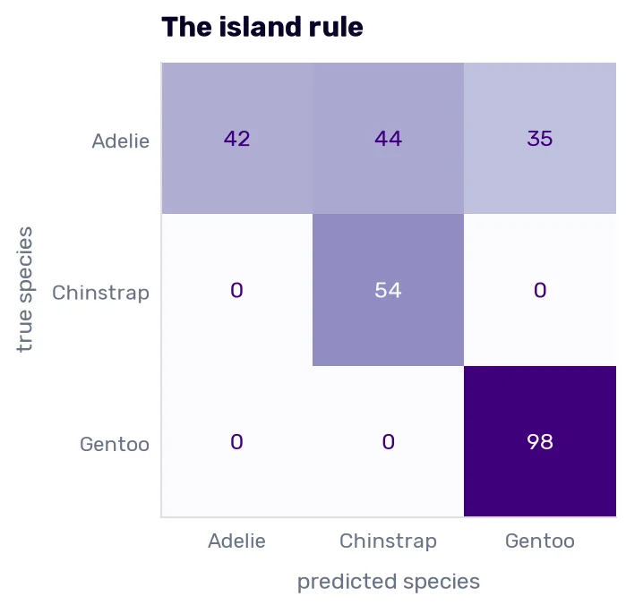
The correct answers sit on the diagonal: 42 + 54 + 98 = 194. Everything off the diagonal is a mistake, and here all 79 of them are in the first row. The rule finds every Chinstrap and every Gentoo. Of the 121 Adelies, it gets the 42 on Torgersen right. It calls the 44 on Dream “Chinstrap” and the 35 on Biscoe “Gentoo”.
Now, read the matrix by columns. Whenever the rule says “Adelie”, it’s right, 42 times out of 42. When it says “Chinstrap”, it’s right 54 times out of 98.
A 71% accuracy could also belong to a model that confuses every species with every other one a little. The two models would need different repairs, and the accuracy can’t tell them apart. The matrix can, and it also tells you which rows of the data to open first. With normalize='true', every row is divided by its total, which is easier to read when the classes differ in size: the Adelie row becomes 0.35, 0.36, and 0.29.
One question at a time
Most of the vocabulary of classification metrics was made for questions with two answers. A problem with three classes contains three such questions, so let’s take one: is this penguin a Chinstrap?
The class we are looking for is called the positive class, and everything else is negative. Nothing about the word means “good.” In a model that detects fraud, the fraud is the positive class. I guess that after COVID-19 everyone understands that a positive result of a PCR test doesn’t mean anything good.
For this question, the island rule shrinks to one statement: a penguin on Dream is a Chinstrap.
is_chinstrap = species == 'Chinstrap'
on_dream = train_df['island'] == 'Dream'

pd.crosstab(is_chinstrap.rename('is a Chinstrap'), on_dream.rename('said Chinstrap'))
| is a Chinstrap | False | True |
|---|---|---|
| False | 175 | 44 |
| True | 0 | 54 |
The rows are the truth, and the columns are what the rule said.
Each of the four cells has a name:
- 54 true positives: Chinstraps the rule called Chinstraps
- 44 false positives: Adelies from Dream the rule called Chinstraps
- 0 false negatives: Chinstraps the rule missed
- 175 true negatives: other penguins the rule correctly left alone
Pandas sorts the labels the way scikit-learn does, and False comes before True. The true negatives land in the top-left corner, where many textbooks draw the true positives. (When you need the four numbers in code, confusion_matrix(is_chinstrap, on_dream).ravel() returns them as true negatives, false positives, false negatives, true positives.)
How accurate is our classifier? Before we answer, let’s add a second classifier, one that never says “Chinstrap”.
never = np.zeros(len(train_df), dtype=bool)

pd.Series({
    'never a Chinstrap': accuracy_score(is_chinstrap, never),
    'Dream means Chinstrap': accuracy_score(is_chinstrap, on_dream),
}, name='accuracy').round(3)
| accuracy | |
|---|---|
| never a Chinstrap | 0.802 |
| Dream means Chinstrap | 0.839 |
A classifier that can’t find a single Chinstrap is 80% accurate, because 219 of the 273 penguins aren’t Chinstraps and it gets all of them for free. The rule that finds every Chinstrap scores 84%. The whole difference between useless and useful is 10 penguins out of 273, less than 4 percentage points.
The true negatives do that. They are the easy answers, and the rarer the positive class, the more of them there are. If one penguin in 100 were a Chinstrap, “never a Chinstrap” would be 99% accurate. This is what happened to the news filter in the machine learning process: the accuracy counted both kinds of mistakes as equal, and we cared about one of them far more than the other. Rare classes get a chapter of their own later. For now, we need numbers that leave the true negatives out.
Precision and recall
Imagine a radar. It looks at a point in the sky and says “plane” or “empty”, so it’s a classifier, and the planes are the positive class. (I borrowed the radar from my article about precision and recall.)
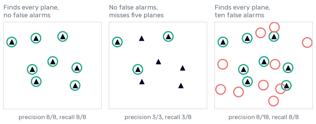
The first radar reports all eight planes and nothing else. The second one never raises a false alarm, and it misses five planes. If those are enemy planes, we have a problem. The third one finds every plane and adds 10 reports of planes that aren’t there. We scramble the fighters 18 times and burn a lot of jet fuel chasing nothing.
Precision answers the question “when the classifier says yes, how often is it right?”
\[\mathrm{precision} = \frac{\mathrm{true\ positives}}{\mathrm{true\ positives} + \mathrm{false\ positives}}\]Recall answers “of all the real positives, how many did the classifier find?”
\[\mathrm{recall} = \frac{\mathrm{true\ positives}}{\mathrm{true\ positives} + \mathrm{false\ negatives}}\]The second radar has a precision of 3/3 and a recall of 3/8. The third one has a recall of 8/8 and a precision of 8/18. Neither formula contains the true negatives, so the empty sky no longer earns any points.
Back to the penguins:
from sklearn.metrics import precision_score, recall_score

is_adelie = species == 'Adelie'
on_torgersen = train_df['island'] == 'Torgersen'

pd.DataFrame({
    'precision': [precision_score(is_chinstrap, on_dream), precision_score(is_adelie, on_torgersen)],
    'recall': [recall_score(is_chinstrap, on_dream), recall_score(is_adelie, on_torgersen)],
}, index=['Dream means Chinstrap', 'Torgersen means Adelie']).round(2)
| precision | recall | |
|---|---|---|
| Dream means Chinstrap | 0.55 | 1 |
| Torgersen means Adelie | 1 | 0.35 |
For the Chinstraps, the island rule is the third radar. It finds all 54, and 44 of its 98 reports are false alarms. For the Adelies, the same rule is the second radar: every “Adelie” is an Adelie, and 79 of the 121 Adelies go unreported.
What about the classifier that never says “Chinstrap”? Its recall is 0. Its precision is 0 divided by 0, because it never said yes. Scikit-learn returns 0.0 and warns you:
UndefinedMetricWarning: Precision is ill-defined and being set to 0.0 due to no predicted samples. Use `zero_division` parameter to control this behavior.
Don’t silence that warning before you read it. It usually means the model never predicts one of the classes, which you want to know.
Which of the two numbers matters more? It depends on what each mistake costs, and the code can’t know that. For the radar, a missed plane is worse than a wasted flight, so we want recall and pay for it with precision. The news filter was the same: an article thrown away by mistake never reached a human, and a useless article that got through cost an analyst a minute. A spam filter is the opposite case, because a real email in the spam folder hurts more than one more ad in the inbox.
Either number is easy to max out alone. A classifier that says yes to everything has a recall of 100%. One that says yes a single time, when it is certain, has a precision of 100%. So a precision reported without the recall tells you nothing.
F1: one number made of two
The F1 score is the harmonic mean of the precision and the recall:
\[F_1 = \frac{2 \cdot \mathrm{precision} \cdot \mathrm{recall}}{\mathrm{precision} + \mathrm{recall}}\]Why this mean and not the ordinary one? Take a radar that reports every point in the sky. Its recall is 1, and its precision is close to 0, say 0.01. The ordinary mean of the two is 0.505, which sounds like half of a working radar. The harmonic mean is 0.02. It stays close to the smaller of the two numbers, so a classifier can’t buy a good F1 by maxing out one of them.
from sklearn.metrics import f1_score, fbeta_score

f1_score(is_chinstrap, on_dream)
For “Dream means Chinstrap”, the precision is 0.55, and the recall is 1. Their ordinary mean is 0.78, and the F1 is 0.71.
F1 treats the two numbers as equally important. When they aren’t, there is the Fβ score:
\[F_\beta = \frac{(1 + \beta^2) \cdot \mathrm{precision} \cdot \mathrm{recall}}{\beta^2 \cdot \mathrm{precision} + \mathrm{recall}}\]With β above 1, the recall counts for more. With β below 1, the precision does. fbeta_score(is_chinstrap, on_dream, beta=2) returns 0.86, because the rule’s recall is its strong side, and beta=0.5 returns 0.61. If you want to see what these formulas look like for every pair of precision and recall, I plotted them in the article about the F1 score.
The F1 score can still flatter a model. A classifier that says yes to everything gets a low F1 only when the positive class is rare. Take the sexes of the 264 penguins that had a lab result, and a classifier that calls every penguin a male:
always_male = np.full(len(known), 'MALE')

f1_score(known['sex'], always_male, pos_label='MALE')
The result is 0.67. Half of the penguins are males, so the precision is 0.51, the recall is 1, and the harmonic mean of those two looks respectable.
F1 also changes when you swap the classes. The same always-male classifier, scored with pos_label='FEMALE', gets 0. “Dream means Chinstrap” gets 0.71 for finding Chinstraps and 0.89 for finding everything else. The true negatives aren’t in the formula, so it matters which class you call positive, and you have to say which one you mean every time you report an F1.
And a low F1 doesn’t say whether the problem is false positives or false negatives. To find out, you go back to the confusion matrix.
Three classes, one number
The penguins have three species, so every one of these metrics exists three times, once per species. Scikit-learn prints all of them at once:
from sklearn.metrics import classification_report

print(classification_report(species, by_island))
              precision    recall  f1-score   support

      Adelie       1.00      0.35      0.52       121
   Chinstrap       0.55      1.00      0.71        54
      Gentoo       0.74      1.00      0.85        98

    accuracy                           0.71       273
   macro avg       0.76      0.78      0.69       273
weighted avg       0.82      0.71      0.67       273
The support column is the number of penguins of each species. The three rows at the top are the three yes-or-no questions, each with its own species as the positive class.
The two rows at the bottom squeeze each column into one number, in two different ways. The macro average is the plain mean of the three rows, so every species counts the same, no matter how many penguins it has. The weighted average multiplies each row by its support first, so the Adelies count more than twice as much as the Chinstraps.
Which one do you want? If a rare class matters as much as a common one, the macro average. The weighted one lets a model do badly on a small class without the number moving much, which is the accuracy’s problem again.
The macro average of the recall has its own name, the balanced accuracy. Here are the dummy and the island rule on four metrics:
from sklearn.metrics import balanced_accuracy_score, matthews_corrcoef

pd.DataFrame({
    name: {
        'accuracy': accuracy_score(species, guesses),
        'balanced accuracy': balanced_accuracy_score(species, guesses),
        'macro F1': f1_score(species, guesses, average='macro', zero_division=0),
        'MCC': matthews_corrcoef(species, guesses),
    }
    for name, guesses in {'always Adelie': always_adelie, 'the island rule': by_island}.items()
}).T.round(2)
| accuracy | balanced accuracy | macro F1 | MCC | |
|---|---|---|---|---|
| always Adelie | 0.44 | 0.33 | 0.2 | 0 |
| the island rule | 0.71 | 0.78 | 0.69 | 0.64 |
The dummy’s accuracy is 44% only because the Adelies happen to be the largest species. Its balanced accuracy is 33%: a recall of 1 for the Adelies and 0 for the other two. Any classifier that always gives the same answer gets exactly one in three here, however lopsided the classes are, which makes the balanced accuracy easy to judge without looking up the class sizes.
The island rule goes the other way, from 71% to 78%. All of its mistakes are in the biggest class, and the balanced accuracy counts that class as one third of the score instead of 44% of it.
The last column is the Matthews correlation coefficient (MCC). It’s computed from the whole confusion matrix, the true negatives included, and it runs from −1 to 1. A perfect classifier gets 1, one that does no better than chance gets 0 (scikit-learn also returns 0 for a classifier that always gives the same answer), and one that is wrong more often than chance goes below 0. When you need a single number and can’t say which class is the positive one, the MCC is a good choice, as long as you don’t have to explain it to anyone.
Scores and thresholds
So far, every classifier gave a flat answer. Most models can say more than that. The sex classifier from Nearest neighbors that vote asks five neighbors, and the answer we have been scoring is the majority of the five. Here is its confusion matrix, from the cross-validated predictions we already have:
confusion_matrix(known['sex'], predicted)
array([[118,  12],
       [ 10, 124]])
Females come first in the alphabet. The model called 12 females males and 10 males females. Let’s get the precision:
precision_score(known['sex'], predicted)
ValueError: pos_label=1 is not a valid label. It should be one of ['FEMALE' 'MALE']
Scikit-learn assumes that the positive class is called 1. With text labels, it refuses to guess, and I’m glad it does, because we have just seen that the F1 for one class can be 0.67 while the F1 for the other is 0. I will take the males as the positive class. With pos_label='MALE', the precision is 0.91 (124 of the 136 penguins called male), and the recall is 0.93 (124 of the 134 males).
Now, the votes themselves. predict_proba() returns the share of the neighbors that voted for each class:
is_male = (known['sex'] == 'MALE').to_numpy()

male_share = cross_val_predict(knn, known[numeric], known['sex'], cv=folds, method='predict_proba')[:, 1].round(1)

votes = pd.crosstab(pd.Series(male_share, name='share of male neighbors'), known['sex'].to_numpy(), colnames=[None])
votes
| share of male neighbors | FEMALE | MALE |
|---|---|---|
| 0 | 80 | 1 |
| 0.2 | 29 | 3 |
| 0.4 | 9 | 6 |
| 0.6 | 10 | 16 |
| 0.8 | 1 | 25 |
| 1 | 1 | 83 |
positions = np.arange(len(votes))
fig, ax = plt.subplots()
ax.bar(positions - 0.19, votes['FEMALE'], 0.38, label='females', color='#eb6834')
ax.bar(positions + 0.19, votes['MALE'], 0.38, label='males', color='#4d41e0')
ax.set_xticks(positions, votes.index)
ax.set_xlabel('share of male neighbors')
ax.set_ylabel('penguins')
ax.set_title('What the five neighbors said')
ax.legend()
plt.show()
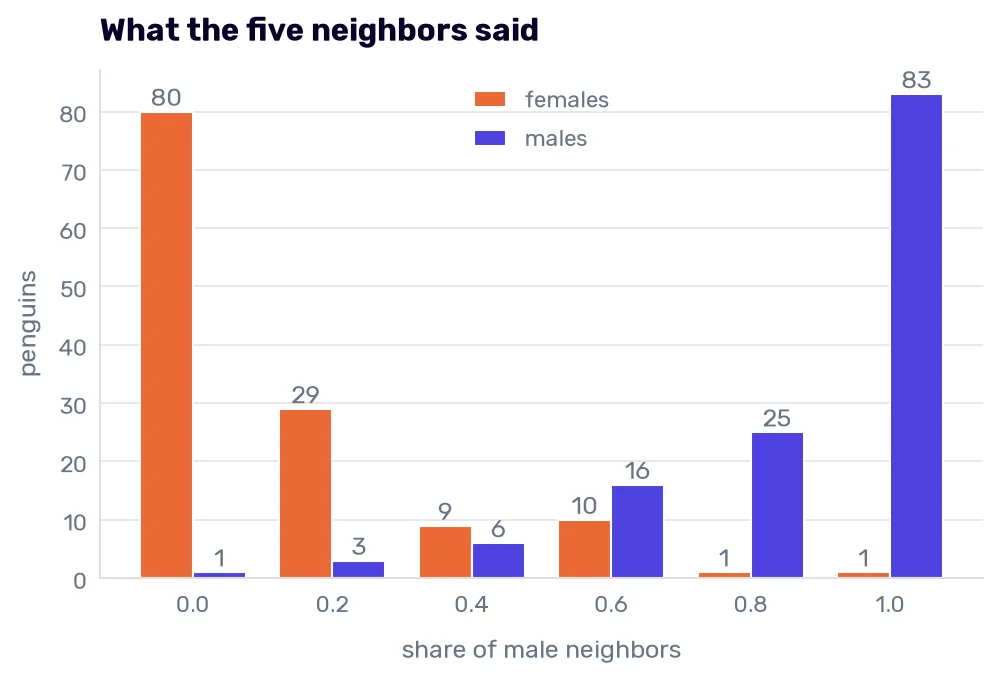
With five neighbors, there are only six possible scores. At both ends, the neighbors agree and are nearly always right. The mistakes are in the middle: of the 41 penguins with a 3-to-2 vote either way, 16 got the wrong answer.
predict() says “male” when more than half of the neighbors do. That is a threshold of 0.5, and nobody chose it. We can put it anywhere:
rows = []
for threshold in [0.1, 0.3, 0.5, 0.7, 0.9]:
    said_male = male_share > threshold
    rows.append({
        'threshold': threshold,
        'said male': said_male.sum(),
        'females among them': (said_male & ~is_male).sum(),
        'males missed': (~said_male & is_male).sum(),
        'precision': precision_score(is_male, said_male),
        'recall': recall_score(is_male, said_male),
        'accuracy': accuracy_score(is_male, said_male),
    })

pd.DataFrame(rows).set_index('threshold').round(3)
| threshold | said male | females among them | males missed | precision | recall | accuracy |
|---|---|---|---|---|---|---|
| 0.1 | 183 | 50 | 1 | 0.727 | 0.993 | 0.807 |
| 0.3 | 151 | 21 | 4 | 0.861 | 0.97 | 0.905 |
| 0.5 | 136 | 12 | 10 | 0.912 | 0.925 | 0.917 |
| 0.7 | 110 | 2 | 26 | 0.982 | 0.806 | 0.894 |
| 0.9 | 84 | 1 | 51 | 0.988 | 0.619 | 0.803 |
It’s one model, and nothing was retrained between the rows. At 0.7, it needs four male neighbors out of five. It then says “male” 110 times and is wrong twice, at the price of 26 males it no longer reports. At 0.1, one male neighbor is enough, and it misses a single male while calling 50 females males. Every row down the table has a higher precision and a lower recall. Nothing in the model says which row to use, so we have to pick one.
Here, the accuracy is best at 0.5, because a penguin with more male neighbors than female ones is more likely to be a male, and I counted both mistakes as equal. When the mistakes cost different amounts, the best threshold moves. The news filter used 0.85 for some languages (see the evaluation step).
The scores allow one more thing: the model can decline to answer. Suppose a lab test is expensive, and we want to test as few penguins as we can. We could accept the model’s answer when at least four of the five neighbors agree and send the other 41 penguins to the lab. Of the 223 answers we keep, six are wrong. The accuracy on them is 97% instead of 92%, and the lab does 16% of the work.
For moving the threshold, scikit-learn has two wrappers. (Neither can decline to answer. For that, you compare the scores with your own limits.) FixedThresholdClassifier(knn, threshold=0.7, pos_label='MALE') is a classifier whose predict() uses your threshold. TunedThresholdClassifierCV picks the threshold for a metric you name, using cross-validation inside the training data.
Wherever the threshold comes from, it’s a decision like any other, so it’s made on validation data. If you tune it on the test set, you have used one of the looks Rule 14 allows.
With three classes, predict() has no threshold to use and answers with the class that has the highest score. The threshold comes back as soon as you ask a yes-or-no question about one class.
ROC and AUC
A threshold table describes a model at five settings. Can we compare two models at every setting at once?
The radar returns here, because radar engineers had this problem first. An operator can turn the sensitivity of a receiver up and see more planes along with more noise, or turn it down and see less of both. The curve that shows the whole trade is called the receiver operating characteristic, the ROC curve, and the name is from the 1940s.
The true positive rate is the recall under another name: the share of the males the model finds. The false positive rate is the share of the females it calls male. roc_curve() computes both for every threshold that changes anything:
from sklearn.metrics import roc_auc_score, roc_curve

false_positive_rate, true_positive_rate, thresholds = roc_curve(is_male, male_share)

pd.DataFrame({
    'threshold': thresholds,
    'false positive rate': false_positive_rate,
    'true positive rate': true_positive_rate,
}).round(3)
| threshold | false positive rate | true positive rate | |
|---|---|---|---|
| 0 | inf | 0 | 0 |
| 1 | 1 | 0.008 | 0.619 |
| 2 | 0.8 | 0.015 | 0.806 |
| 3 | 0.6 | 0.092 | 0.925 |
| 4 | 0.4 | 0.162 | 0.97 |
| 5 | 0.2 | 0.385 | 0.993 |
| 6 | 0 | 1 | 1 |
Here, a penguin is called male when its score is at least the threshold, so the row for 0.6 is our 0.5 row from before: 12 of the 130 females and 124 of the 134 males. The first row is a threshold nobody can reach, so nobody is called male. The last row calls everybody male.
Before I draw it, I want a second score to compare with. A score doesn’t have to come from a model. Males are heavier, so the body mass in grams is a score for “is it a male?” as well.
mass_fpr, mass_tpr, _ = roc_curve(is_male, known['body_mass_g'])

fig, ax = plt.subplots(figsize=(6, 5.6))
ax.plot(false_positive_rate, true_positive_rate, marker='o', label='five neighbors, AUC 0.97')
ax.plot(mass_fpr, mass_tpr, label='body mass alone, AUC 0.75')
ax.plot([0, 1], [0, 1], linestyle='--', color='#687385', label='a coin, AUC 0.50')
ax.set_xlabel('false positive rate (females called male)')
ax.set_ylabel('true positive rate (males found)')
ax.set_title('Two ROC curves for "is it a male?"')
for rate, found, threshold in zip(false_positive_rate[1:-1], true_positive_rate[1:-1], thresholds[1:-1]):
    ax.annotate(f'{threshold:.1f}', (rate, found), textcoords='offset points', xytext=(8, -12))
ax.legend(loc='lower right')
plt.show()
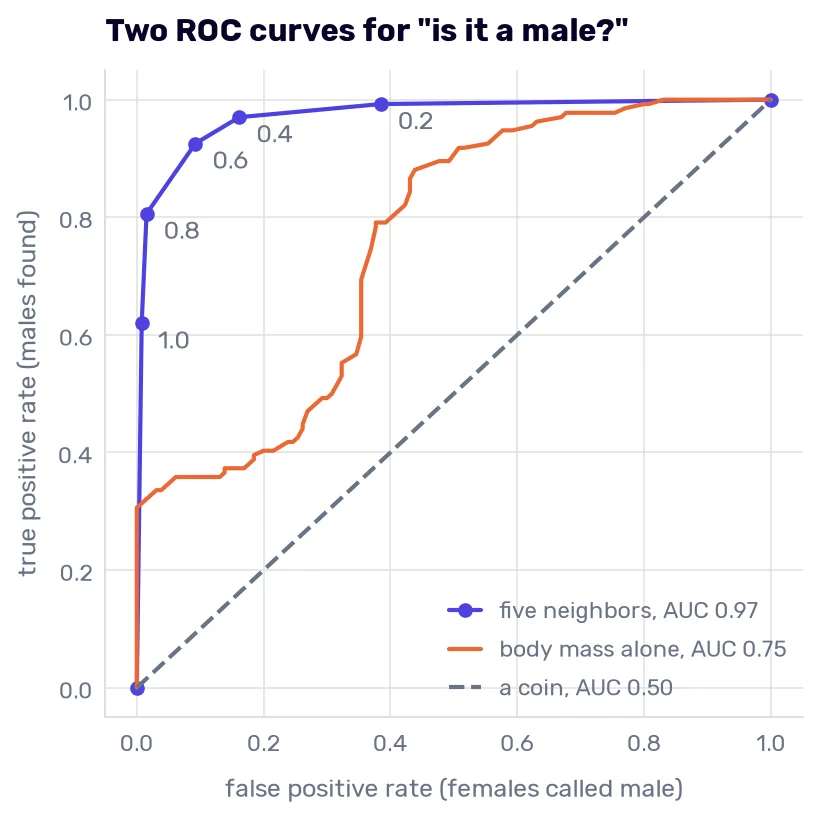
Every point is one threshold. (The dots on the upper curve are the rows of the table.) A perfect model would sit in the top-left corner: all the males found, no female called male. A model that flips a coin walks along the diagonal, because it finds the same share of the males as of the females. The closer a curve gets to the corner, the better the trade it offers at every threshold.
The AUC is the area under the curve. It’s 1 for the perfect model, 0.5 for the coin, 0.97 for the neighbors, and 0.75 for the body mass.
What does 0.75 mean? It’s tempting to read it as “right 75% of the time,” and that’s wrong. To be right or wrong, a model needs a threshold, and the AUC never picks one. We can compute what it measures by hand. Pair every male with every female and count the pairs in which the male is the heavier bird:
males = known.loc[is_male, 'body_mass_g'].to_numpy()
females = known.loc[~is_male, 'body_mass_g'].to_numpy()

heavier = (males[:, None] > females).mean()
same = (males[:, None] == females).mean()

np.round([heavier, same, heavier + same / 2, roc_auc_score(is_male, known['body_mass_g'])], 4)
array([0.7498, 0.0086, 0.7541, 0.7541])
There are 17,420 pairs. The male is heavier in 74.98% of them, and the two weigh the same in 0.86%. Count a tie as half, and you get 0.7541, which is the AUC to the last digit. The AUC is the chance that a randomly picked positive gets a higher score than a randomly picked negative. It tells you how well a score sorts the rows, which is why it’s good for comparing models before anyone has chosen a threshold. (I explain it with cats and dogs in the article about ROC and AUC.)
The orange curve has a strange shape, flat in the middle. This is Rule 22 again, the one about correlations across mixed groups:
known.assign(is_male=is_male).groupby('species', observed=True).apply(
    lambda penguins: roc_auc_score(penguins['is_male'], penguins['body_mass_g']), include_groups=False
).rename('AUC').round(2)
| species | AUC |
|---|---|
| Adelie | 0.94 |
| Chinstrap | 0.83 |
| Gentoo | 0.99 |
Inside every species, the body mass sorts the sexes far better than the 0.75 says. Among the Gentoos, it’s almost perfect. The pooled number is low because most of the 17,420 pairs put a male of one species next to a female of another, and an average female Gentoo (4684 g) outweighs an average male Adelie (4060 g) by a wide margin. The AUC of a score across mixed groups can be far from its AUC inside each of them, in either direction. If your model will be used one group at a time, like the news filter with a model per language, compute the AUC per group.
The AUC also has the limits we saw in the machine learning process. It averages over every threshold, including the ones you would never ship, so two models with the same AUC can differ a lot at the one threshold you use. And it knows nothing about costs. Nothing in the curve says that a missed plane is worse than a wasted flight.
There is a sibling curve, the precision-recall curve, which plots those two numbers for every threshold (PrecisionRecallDisplay draws it). It matters when the positive class is rare. The false positive rate is divided by the number of negatives, and with enough negatives it stays tiny even when the false alarms outnumber the hits. Precision is divided by the number of reports, so every false alarm lowers it. We will need this curve in the chapter about rare classes.
Is the score a probability?
We have been using the share of male neighbors to sort penguins. Can we also believe it as a number? If the model says 0.6, are 60% of such penguins male?
votes.assign(
    penguins=votes.sum(axis=1),
    males=(votes['MALE'] / votes.sum(axis=1)).round(2),
)[['penguins', 'males']]
| share of male neighbors | penguins | males |
|---|---|---|
| 0 | 81 | 0.01 |
| 0.2 | 32 | 0.09 |
| 0.4 | 15 | 0.4 |
| 0.6 | 26 | 0.62 |
| 0.8 | 26 | 0.96 |
| 1 | 84 | 0.99 |
In the middle, yes: 40% of the penguins with a score of 0.4 are males, and 62% of those with 0.6. A score like that is called calibrated. At 0.2 and 0.8, the model is more modest than it should be. Four neighbors out of five is 80% of the vote, and such penguins are male 96% of the time.
The AUC doesn’t notice any of this. It only looks at the order of the scores, so you could square every score and get the same AUC from numbers that are no longer probabilities. Calibration matters as soon as someone multiplies the score by something, like the cost of a mistake, or compares the scores of two models. That was the problem with the per-language thresholds: a 0.85 from one model isn’t a 0.85 from another.
Two penguins in the table deserve a look: the male with a score of 0 and the female with a score of 1. Five neighbors out of five were wrong about each. A model that says 0 or 1 claims to be certain, and there is a metric, the log loss, that punishes a certain and wrong answer without limit. It scores the probabilities themselves, and the model in the next chapter is trained by minimizing it, so I will explain it there.
How many penguins is one percent?
All of these metrics are fractions, and a fraction hides how many rows stand behind it. In Is the imputer any good?, the five folds scored between 0.887 and 0.943. That looks like a model that swings by almost 6 percentage points depending on the data. In penguins, the five folds got 50, 48, 50, 47, and 47 right, out of 53 (the last fold has 52). The best fold and the worst one are three penguins apart, and a single penguin moves a fold by 1.9 percentage points.
The total has the same problem on a smaller scale. The model got 242 of 264 penguins right. If we had measured a different 264 penguins from the same colonies, we would have gotten a different count. For a share of 92% out of 264, the standard error from your statistics course is 1.7 percentage points, so anything between roughly 88% and 95% would be unsurprising. (Roughly, because the formula assumes independent answers, and the five models that produced ours share most of their training penguins.)
It gets worse on the test set, and worse again per class. We have 69 test penguins, so one penguin is 1.4 percentage points of accuracy. Only 14 of them are Chinstraps. One Chinstrap more or less is 7 percentage points of Chinstrap recall, and the possible values jump from 100% to 93% to 86%.
The penguins are an easy problem, and the species models we are about to train will score in the high nineties. Two models at 97.1% and 98.6% on the test set differ by one penguin. Rule 19 asked us to compare models fold by fold before believing a lead, and here the comparison is 68 penguins against 67.
What we will measure on the penguins
The metric follows from the costs, so it has to be chosen before the model exists. Otherwise, it’s too easy to pick the one on which the model looks best.
For our species question, I can’t name a mistake that is worse than the others. Calling an Adelie a Chinstrap costs the same as calling a Chinstrap a Gentoo, which is nothing, because nobody will use this model. So I will pretend all three species matter equally, and that decides most of it:
- The confusion matrix comes first, every time. It’s nine numbers, and it shows which species get mixed up.
- The recall per species goes next to it, with the number of penguins behind each one.
- When we need a single number to compare two versions of a model, it’s the balanced accuracy. Every species counts the same, and the baselines are easy to remember: 33% for the dummy and 78% for the island rule (Rule 10).
- The accuracy stays in the tables, because the earlier chapters used it and it’s the number everyone asks for first.
We need no threshold, because the model will answer with its highest score.
No model was chosen in this chapter, so we didn’t look at the test set. In the next chapter, we finally train the species model, and when it makes mistakes, the confusion matrix will say which penguins to open first.