
We waited three chapters for a penguin classification model. The waiting is over. We have a clean table of 273 training penguins, and we chose the metric: the confusion matrix first, the recall per species next to it, and the balanced accuracy when two versions need one number. The baselines are 33% for the dummy and 78% for the island rule.
Most of the models in this chapter are old acquaintances. The nearest neighbors, the trees, the forest, and the boosting were all taken apart on the cars, so for each of them I will only say what changes when the answer is a species. One model is new, but not really new. It’s the linear model coming back.
Every model gets scored the same way, so the scoring goes into a function:
from sklearn.metrics import balanced_accuracy_score, log_loss

def fold_scores(model, columns=numeric):
    shares = cross_val_predict(model, train_df[columns], species, cv=folds, method='predict_proba')
    predicted = np.unique(species)[shares.argmax(axis=1)]
    return pd.Series({
        'right': (predicted == species).sum(),
        'accuracy': accuracy_score(species, predicted),
        'balanced accuracy': balanced_accuracy_score(species, predicted),
        'log loss': log_loss(species, shares),
    })
folds are the five stratified folds from Is the imputer any good?, this time stratified by the species. numeric holds the four measurements. The island and the sex stay out until the end of the chapter. The function asks every model for its scores (predict_proba()) and takes the species with the highest one, which is what predict() does. It counts the penguins it got right, because Rule 25 asked for the count next to every percentage.
Nearest neighbors, three species
We already have a classifier. In Nearest neighbors that vote, five neighbors voted on a penguin’s sex. Nothing in the algorithm cares that the vote now has three candidates, so the only thing to choose is k:
neighbors = {}
for k in [1, 3, 5, 10, 20, 40]:
    scaled = fold_scores(make_pipeline(StandardScaler(), KNeighborsClassifier(n_neighbors=k)))
    unscaled = fold_scores(KNeighborsClassifier(n_neighbors=k))
    neighbors[k] = {
        'right, scaled': scaled['right'],
        'balanced accuracy, scaled': scaled['balanced accuracy'],
        'right, unscaled': unscaled['right'],
        'balanced accuracy, unscaled': unscaled['balanced accuracy'],
    }

pd.DataFrame(neighbors).T.rename_axis('k').round(3)
| k | right, scaled | balanced accuracy, scaled | right, unscaled | balanced accuracy, unscaled |
|---|---|---|---|---|
| 1 | 267 | 0.97 | 217 | 0.759 |
| 3 | 268 | 0.976 | 210 | 0.712 |
| 5 | 269 | 0.975 | 207 | 0.688 |
| 10 | 268 | 0.969 | 202 | 0.63 |
| 20 | 267 | 0.963 | 199 | 0.628 |
| 40 | 266 | 0.96 | 198 | 0.602 |
With the scaler, five neighbors get 269 of the 273 penguins right. That’s a balanced accuracy of 97.5%, against 78% for the island rule.
Look at how little k matters (in this case. It’s not a general rule!). From 1 neighbor to 40, the count moves between 266 and 269. I keep k=5 because it’s the default and nothing in the table argues against it.
The scaler matters a lot. Without it, the same five neighbors get 207 right. That’s 13 more than the island rule’s 194, and it’s still the worse model by the metric we chose: a balanced accuracy of 69% against the rule’s 78%. In Models that don’t draw lines, the unscaled model won, because the column that took over the distance was the weight, the best column the cars had. In Before the first model, I said the penguins would go the other way: the body mass has a standard deviation of 806 g, the bill depth of 2.0 mm, and the mass can’t tell an Adelie from a Chinstrap. The unscaled model finds 18 of the 54 Chinstraps.
Here is the confusion matrix of the scaled model:
species_knn = make_pipeline(StandardScaler(), KNeighborsClassifier(n_neighbors=5))
confusion_matrix(species, cross_val_predict(species_knn, train_df[numeric], species, cv=folds))
array([[121,   0,   0],
       [  4,  50,   0],
       [  0,   0,  98]])
Every Adelie and every Gentoo is right. All four mistakes are Chinstraps that the model calls “Adelie”, so the recall is 100% for two species and 93% (50 of 54) for the third. We will open those four rows later in the chapter.
KNeighborsClassifier has one more setting you will see in tutorials. With weights='distance', a close neighbor’s vote counts more than a distant one’s. (The regressor has the same setting, and there it turns the average into a weighted average.) On the penguins, it gets 268 instead of 269, so I leave it alone.
Which measurements decide?
Nearest neighbors have no coefficients and no feature_importances_. The method from Which columns do the trees use? works on any model, though. We shuffle one column in the validation part of a fold and see how much the score drops. The score is now the balanced accuracy:
def fold_importance(model):
    importances = []
    for train_rows, validation_rows in folds.split(train_df, species):
        fitted = clone(model).fit(train_df[numeric].iloc[train_rows], species.iloc[train_rows])
        result = permutation_importance(
            fitted, train_df[numeric].iloc[validation_rows], species.iloc[validation_rows],
            scoring='balanced_accuracy', n_repeats=30, random_state=42,
        )
        importances.append(pd.Series(result.importances_mean, index=numeric))
    return pd.DataFrame(importances, index=range(1, 6)).T.assign(mean=lambda table: table.mean(axis=1))

fold_importance(species_knn).sort_values('mean', ascending=False).round(3)
| 1 | 2 | 3 | 4 | 5 | mean | |
|---|---|---|---|---|---|---|
| culmen_length_mm | 0.273 | 0.34 | 0.345 | 0.227 | 0.346 | 0.306 |
| culmen_depth_mm | 0.155 | 0.262 | 0.17 | 0.095 | 0.201 | 0.177 |
| body_mass_g | 0.093 | 0.053 | 0.054 | 0.045 | 0.063 | 0.062 |
| flipper_length_mm | 0.047 | 0.029 | 0.03 | 0.017 | 0.028 | 0.03 |
Shuffling the bill length takes 31 percentage points off the balanced accuracy, and the bill depth costs 18. The order is the same in all five folds.
The flipper is last, which looks wrong at first. In The flipper has two peaks, it was the column that separated the Gentoos from everybody else. It still does. But a Gentoo’s bill is 14.9 mm deep on average, and the other two species have 18.4 mm and 18.5 mm, so the bill depth separates the Gentoos too. When the flipper is shuffled, the model still has the depth (and the mass) to recognize a Gentoo by. Permutation importance measures what the model loses without a column while it keeps all the others, so shuffling a column that has a stand-in costs little. It’s the same trade as in Rule 15, where correlated columns shared their coefficients.
The map of a classifier
Two columns carry most of the decision, and two columns fit on a chart. So let’s train the same model on the bill length and the bill depth alone, ask it about every point of the chart, and color the point with the answer:
from sklearn.inspection import DecisionBoundaryDisplay

bill = ['culmen_length_mm', 'culmen_depth_mm']

def species_regions(model, title, ax=None):
    ax = ax or plt.gca()
    fitted = clone(model).fit(train_df[bill], species)
    DecisionBoundaryDisplay.from_estimator(
        fitted, train_df[bill], response_method='predict', plot_method='pcolormesh', grid_resolution=400,
        multiclass_colors=list(SPECIES_COLORS.values()), alpha=0.25, ax=ax,
    )
    for name, color in SPECIES_COLORS.items():
        rows = train_df[species == name]
        ax.scatter(rows[bill[0]], rows[bill[1]], color=color, label=name, s=22)
    ax.grid(False)
    ax.set_title(title, loc='left')
    ax.set_xlabel('bill length [mm]')
    ax.set_ylabel('bill depth [mm]')

species_regions(species_knn, 'What five neighbors say about every bill')
plt.legend()
plt.show()
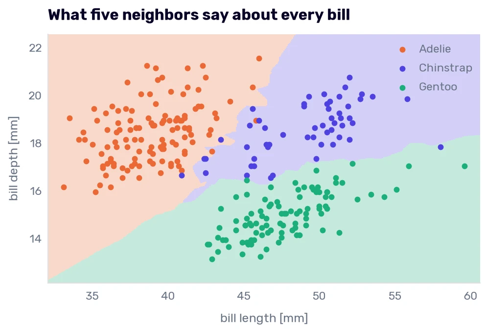
A classifier cuts the space of its inputs into regions, one or more per class. The lines between the regions are called decision boundaries. The dots are the training penguins, and a dot on a background of another color is a penguin that gets outvoted even with its own vote counted.
The model in the chart is a second model. It has two columns, and the one we scored has four, whose regions I can’t draw in two dimensions. On the folds, the two-column model gets 265 right (95.7% balanced), so the flipper and the body mass together were worth four penguins.
The boundaries are ragged, because every stretch of them is decided by the handful of penguins that happen to live there. Near the bottom of the Adelie cloud, a narrow indigo tongue reaches down between the Adelies and the Gentoos. A few Chinstraps with short bills made it. The Adelies and the Chinstraps meet along a border that runs from a bill of 41 mm to a bill of 46 mm, roughly the range I named at the end of The classification problem.
Logistic regression
The second model is the linear regression’s sibling, and despite the name it classifies. It keeps the part we know from Inside the linear regression: multiply every column by a coefficient, add them up, add an intercept. With three species, it does this three times, so every penguin gets three scores, one per species:
\[s_k = b_k + a_{k,1} x_1 + a_{k,2} x_2 + \dots + a_{k,p} x_p\]A score can be any number, negative ones included. To turn three scores into three probabilities, the model raises \(e\) to each score, which makes it positive, and divides by the total, which makes the three sum to 1:
\[p_k = \frac{e^{s_k}}{e^{s_1} + e^{s_2} + e^{s_3}}\]The answer is the species with the highest probability, and that’s always the one with the highest score.
from sklearn.linear_model import LogisticRegression

logistic = make_pipeline(StandardScaler(), LogisticRegression())
logistic.fit(train_df[numeric], species)

coefficients = pd.DataFrame(logistic[-1].coef_, index=logistic[-1].classes_, columns=numeric)
coefficients.assign(intercept=logistic[-1].intercept_).round(2)
| culmen_length_mm | culmen_depth_mm | flipper_length_mm | body_mass_g | intercept | |
|---|---|---|---|---|---|
| Adelie | -2.57 | 1.45 | -0.58 | 0.42 | 0.44 |
| Chinstrap | 2.19 | 0.27 | -0.6 | -1.43 | -0.07 |
| Gentoo | 0.39 | -1.72 | 1.18 | 1.01 | -0.37 |
That table is the whole model: 12 coefficients and 3 intercepts. (For running inside a washing machine, add the scaler’s four means and four standard deviations.) The columns are standardized, so a coefficient says what one standard deviation of a measurement does to a score.
A long bill lowers the Adelie score (−2.57) and raises the Chinstrap score (2.19). A deep bill lowers the Gentoo score (−1.72). A Chinstrap is a bird with a long bill on a light body (−1.43 for the mass). All of it agrees with the averages we looked at in Bigger penguins, which is the check Rule 12 asked for.
Rule 15 still applies: the flipper and the mass are correlated, so the two share an effect, and how they split it would change with the rows. And look down any column: −2.57, 2.19, and 0.39 sum to 0 (the same in every column, up to rounding). The probabilities depend only on the differences between the scores, so a coefficient means something only next to the other two in its column.
Let’s follow one penguin through the model. Row 206 is a Chinstrap female with a bill of 42.5 mm by 17.3 mm, a flipper of 187 mm, and a mass of 3350 g:
standardized = logistic[0].transform(train_df.loc[[206], numeric])[0]
scores = coefficients @ standardized + logistic[-1].intercept_
pd.DataFrame({'score': scores, 'probability': np.exp(scores) / np.exp(scores).sum()}).round(3)
| score | probability | |
|---|---|---|
| Adelie | 1.388 | 0.48 |
| Chinstrap | 1.455 | 0.513 |
| Gentoo | -2.843 | 0.007 |
The model is sure she isn’t a Gentoo and can’t decide between the other two. logistic.predict_proba() returns the same three numbers. For the Adelie in row 0, the first row of the file, it returns 0.99, 0.01, and 0.00.
Where is the border between two species? At the points where their scores are equal. Each score is a sum of columns times coefficients, so “equal scores” is a linear equation, and its solutions form a straight line (a flat surface, with four columns):
species_regions(logistic, 'Logistic regression draws straight borders')
plt.legend()
plt.show()
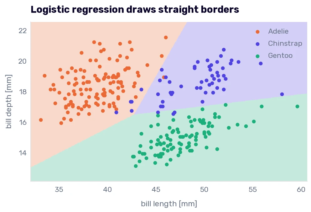
Three straight borders, meeting in one point. No tongues and no islands, however the training penguins are arranged, because the model has nothing to draw them with. That’s the classification version of high bias, and on these penguins it costs nothing:
pd.DataFrame({'nearest neighbors': fold_scores(species_knn), 'logistic regression': fold_scores(logistic)}).T.round(3)
| right | accuracy | balanced accuracy | log loss | |
|---|---|---|---|---|
| nearest neighbors | 269 | 0.985 | 0.975 | 0.033 |
| logistic regression | 269 | 0.985 | 0.979 | 0.06 |
Both get 269 of 273. The logistic regression misses three Chinstraps and one Adelie, the neighbors miss four Chinstraps, and that’s the entire difference in the balanced accuracy.
How it learns, and the log loss
The linear regression had a formula for the best coefficients. The logistic regression has none. It starts with all coefficients at 0 and improves them step by step until the steps stop helping, which is why it has a max_iter setting and the linear regression doesn’t.
“Improves” needs a number to improve, and counting the correct answers won’t do. If a small change to a coefficient moves a probability from 0.48 to 0.49, the answer stays the same, the count stays the same, and the model can’t tell that it’s moving in the right direction. So it is trained on a number that reacts to every such change. For each penguin, take the probability the model gave to the true species and take the negative logarithm of it. The average over all penguins is the log loss (the name cross-entropy means the same thing):
\[\text{log loss} = -\frac{1}{n} \sum_{i=1}^{n} \log p_{i,\,\text{true species of } i}\]A probability of 0.9 for the right species costs 0.11. A coin toss between two species, 0.5, costs 0.69. Giving the right species 0.1 costs 2.3, and 0.01 costs 4.6. A probability of 0 would cost infinity. Scikit-learn clips it at a very small number instead, which makes it 36.
Unlike everything in the metrics chapter, the log loss scores the probabilities themselves, so a model can lose points while being right. It has no fixed scale, but it has a baseline. A dummy that answers every penguin with the shares of the three species in the training data (44%, 20%, and 36%) gets 1.05.
Now, we can read the last column of the tables. With one neighbor, the nearest-neighbors model gets 267 penguins right, and fold_scores gives it a log loss of 0.79. A single neighbor gives its species a share of 1 and the other two a share of 0, so each of the six mistakes costs 36, and 6 × 36 / 273 is 0.79. The model is 98% accurate and, by this metric, not far ahead of a dummy that knows nothing about bills. With five neighbors, the log loss is 0.033, because the true species never got zero votes.
This is the reason I postponed the log loss in Is the score a probability?. It’s the metric to watch when somebody will use the probabilities as numbers. We decided to judge the species model by its answers, so the log loss stays in the tables as a warning light for models that are sure and wrong.
The scaler, again
What happens without the scaler?
LogisticRegression().fit(train_df[numeric], species)
ConvergenceWarning: lbfgs failed to converge after 100 iteration(s) (status=1):
STOP: TOTAL NO. OF ITERATIONS REACHED LIMIT

Increase the number of iterations to improve the convergence (max_iter=100).
You might also want to scale the data as shown in:
    https://scikit-learn.org/stable/modules/preprocessing.html
Please also refer to the documentation for alternative solver options:
    https://scikit-learn.org/stable/modules/linear_model.html#logistic-regression
The step-by-step search ran out of its 100 steps. With grams next to millimeters, a good step size for one coefficient is a terrible one for another, and the search crawls. If you raise max_iter to 10,000, it finishes after 1,690 steps and gets 267 penguins right. The scaled version needs 11 steps and gets 269. Raising max_iter makes the warning go away, but the message itself names the better fix.
The penalty you didn’t ask for
There is a second reason for the scaler. Scikit-learn’s LogisticRegression is regularized by default. It adds the squared coefficients to the number it minimizes, like the Ridge regression in Regularization and tuning, and a penalty on coefficients punishes columns for their units.
The setting is called C, and it works the opposite way from Ridge’s alpha. C multiplies the penguins’ losses where alpha multiplied the penalty, so a small C means a strong penalty, and C=np.inf turns it off. The default is 1. (It multiplies the sum of the losses, and the log loss is their average. The same C is therefore a weaker penalty on a bigger table.)
strengths = {}
for C in [0.01, 0.1, 1, 10, 100, np.inf]:
    model = make_pipeline(StandardScaler(), LogisticRegression(C=C, max_iter=10_000))
    scores = fold_scores(model)
    fitted = model.fit(train_df[numeric], species)
    strengths[C] = {
        'right, folds': scores['right'],
        'log loss, folds': scores['log loss'],
        'right, training': (fitted.predict(train_df[numeric]) == species).sum(),
        'largest coefficient': np.abs(fitted[-1].coef_).max(),
    }

pd.DataFrame(strengths).T.rename_axis('C').round(3)
| C | right, folds | log loss, folds | right, training | largest coefficient |
|---|---|---|---|---|
| 0.01 | 251 | 0.463 | 253 | 0.469 |
| 0.1 | 266 | 0.162 | 267 | 1.267 |
| 1 | 269 | 0.06 | 270 | 2.575 |
| 10 | 269 | 0.032 | 272 | 4.998 |
| 100 | 269 | 0.037 | 273 | 9.744 |
| inf | 269 | 0.062 | 273 | 68.13 |
At 0.01, the penalty is so strong that the model barely dares to tell the species apart. From 1 upward, the folds say 269 every time.
Now, look at the last row. Without the penalty, the model gets all 273 training penguins right, and its largest coefficient is 68. In four dimensions, flat borders can separate our three species without a single training mistake. When that happens, an unpenalized logistic regression has no best answer. Doubling every coefficient keeps the borders where they are and pushes every probability closer to 0 or 1, which lowers the log loss on the training data, so the search would double them again, forever. The 68 is where scikit-learn’s stopping rule ended the run. On the folds, the certainty costs: the log loss goes back up to 0.062 with the same 269 correct answers.
So the default penalty protects you from that, and it also changes what you get when you believe you are fitting a “plain” logistic regression. The coefficients we read earlier are smaller than the unpenalized ones would be. If you read coefficients or compare yours with ones from a statistics package that doesn’t penalize, know which C produced them.
C=10 has the best log loss in the table. I’m not switching to it. Every row from 1 upward has the same 269, and the metric we chose is about the answers.
A detour: when no straight line will do
Straight borders were enough for the penguins. The penguins can’t supply a case where straight borders aren’t, so we leave them for a moment and use a toy. make_circles generates points on two rings, one inside the other:
from matplotlib.colors import ListedColormap
from sklearn.datasets import make_circles
from sklearn.preprocessing import FunctionTransformer

points, ring = make_circles(n_samples=400, noise=0.1, factor=0.5, random_state=42)
points = pd.DataFrame(points, columns=['x', 'y'])

def to_polar(points):
    return pd.DataFrame({
        'radius': np.sqrt(points['x'] ** 2 + points['y'] ** 2),
        'angle': np.arctan2(points['y'], points['x']),
    })

polar = make_pipeline(FunctionTransformer(to_polar), LogisticRegression())

circle_folds = StratifiedKFold(n_splits=5, shuffle=True, random_state=42)
cross_val_score(LogisticRegression(), points, ring, cv=circle_folds).mean(), cross_val_score(polar, points, ring, cv=circle_folds).mean()
(np.float64(0.4525), np.float64(0.9974999999999999))
On x and y, the logistic regression gets 45% of the points right, a little worse than a coin. No straight line has the inner ring on one side and the outer ring on the other. The second model is the same logistic regression, but before it sees a point, a FunctionTransformer replaces x and y with the distance from the center and the angle. Now it gets 399 of the 400 points right. Its coefficient for the radius is −9.03, and for the angle 0.02: the model learned that only the distance matters.
fig, axes = plt.subplots(1, 2, figsize=(7.6, 3.9), sharey=True)
for ax, model, title in zip(axes, [LogisticRegression(), polar], ['x and y', 'radius and angle']):
    DecisionBoundaryDisplay.from_estimator(
        model.fit(points, ring), points, response_method='predict', plot_method='pcolormesh', grid_resolution=300,
        cmap=ListedColormap(['#eb6834', '#4d41e0']), alpha=0.25, ax=ax,
    )
    ax.scatter(points['x'], points['y'], c=np.where(ring == 1, '#4d41e0', '#eb6834'), s=12)
    ax.set_title(title, loc='left')
    ax.set_aspect('equal')
    ax.grid(False)
axes[1].set_ylabel('')
plt.show()
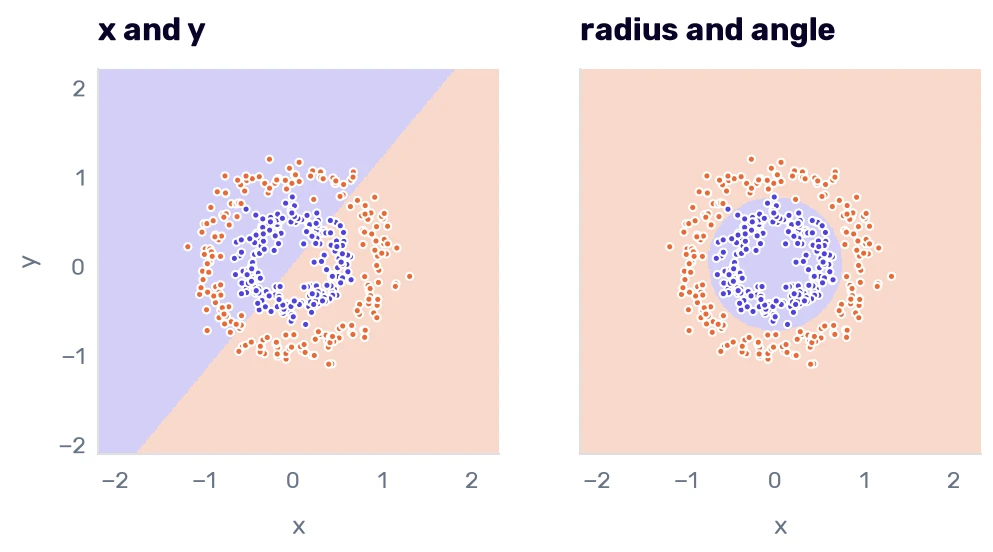
Drawn back on x and y, a straight border in the new columns is a circle. In Improving the model, we changed the coordinates of the target, from miles per gallon to gallons per 100 miles, and a bend became a line. This is the same move on the inputs, at its most extreme: an impossible problem became a trivial one, and the model didn’t change. Mathematics is the closest humanity gets to actual magic (but, as I told you in the intro, remember that ML is not magic).
The trick has a catch. Rule 16 said that a transformation can only rearrange what the columns already hold. Here, they held everything, and I still had to know which rearrangement to ask for. I knew to compute the radius because I knew how the data was made. Real data doesn’t come with a note saying which coordinates it wants. You can let the model search: PolynomialFeatures(degree=2) in front of the same logistic regression gets 99.25%, because x² and y² are among its columns. Or you can use a model that doesn’t draw straight lines in the first place. The five nearest neighbors get 99.25% on the raw x and y. (Kernel methods, such as the support vector machine, build such columns without writing them out. This book doesn’t cover them.)
Back to the penguins.
Trees that ask about the species
The decision tree from Models that don’t draw lines asked yes-or-no questions about one column at a time and picked each question to leave the smallest squared error. A species has no squared error. What does a classification tree minimize?
from sklearn.tree import DecisionTreeClassifier, export_text

small_tree = DecisionTreeClassifier(max_depth=2, random_state=42).fit(train_df[numeric], species)
print(export_text(small_tree, feature_names=numeric, show_weights=True))
|--- flipper_length_mm <= 206.50
|   |--- culmen_length_mm <= 43.35
|   |   |--- weights: [116.00, 4.00, 0.00] class: Adelie
|   |--- culmen_length_mm >  43.35
|   |   |--- weights: [4.00, 45.00, 1.00] class: Chinstrap
|--- flipper_length_mm >  206.50
|   |--- culmen_depth_mm <= 18.00
|   |   |--- weights: [0.00, 0.00, 97.00] class: Gentoo
|   |--- culmen_depth_mm >  18.00
|   |   |--- weights: [1.00, 5.00, 0.00] class: Chinstrap
It wants every box to hold one species. The measure of how mixed a box is has a name, the Gini impurity. It’s the chance that two penguins picked from the box at random (with the first one put back) belong to different species. A box with one species has an impurity of 0. In a formula, with \(p_k\) as the share of species k in the box:
\[\text{Gini} = 1 - \sum_{k} p_k^2\]All 273 training penguins together have an impurity of 0.64. The first question, whether the flipper is longer than 206.5 mm, puts 103 penguins on one side (97 Gentoos, 5 Chinstraps, and 1 Adelie, impurity 0.11) and 170 on the other (120 Adelies, 49 Chinstraps, and 1 Gentoo, impurity 0.42). Weighted by the number of penguins, that’s 0.30, and no other question about any column gets lower. The rest works as it did for the cars: the tree tries every column and every threshold, keeps the best split, and repeats on each side.
A leaf answers with the species most of its penguins have, and the three numbers after weights are what predict_proba() is made of. Our Chinstrap from row 206 (187 mm flipper, 42.5 mm bill) lands in the first box with 116 Adelies and 4 Chinstraps, so the tree calls her an Adelie with a probability of 0.97.
On the cars, I preferred min_samples_leaf to max_depth, and a leaf of 10 cars did best. Let’s see what the penguins say:
trees = {}
for leaf_size in [1, 2, 5, 10, 20, 40]:
    tree = DecisionTreeClassifier(min_samples_leaf=leaf_size, random_state=42)
    fitted = clone(tree).fit(train_df[numeric], species)
    scores = fold_scores(tree)
    trees[leaf_size] = {
        'leaves': fitted.get_n_leaves(),
        'right, training': (fitted.predict(train_df[numeric]) == species).sum(),
        'right, folds': scores['right'],
        'balanced accuracy': scores['balanced accuracy'],
        'log loss': scores['log loss'],
    }

pd.DataFrame(trees).T.rename_axis('min_samples_leaf').round(3)
| min_samples_leaf | leaves | right, training | right, folds | balanced accuracy | log loss |
|---|---|---|---|---|---|
| 1 | 14 | 273 | 264 | 0.957 | 1.188 |
| 2 | 12 | 269 | 263 | 0.951 | 1.192 |
| 5 | 8 | 266 | 257 | 0.92 | 0.737 |
| 10 | 7 | 259 | 256 | 0.917 | 0.778 |
| 20 | 6 | 258 | 256 | 0.917 | 0.808 |
| 40 | 5 | 258 | 254 | 0.915 | 0.359 |
The opposite. The fully grown tree gets the most penguins right (264), and every bigger leaf gets fewer than that. It needs only 14 leaves to get all 273 training penguins right, where the car tree needed 254 leaves to memorize 307 cars. The species are far easier to box than the MPG. The few penguins that take extra questions are the odd Chinstraps and Adelies near the border, and a leaf that must hold 5 or 10 penguins can’t give two odd birds a box of their own, so their neighbors outvote them.
Now, the last column. The fully grown tree has a log loss of 1.19, which is worse than the dummy’s 1.05, at an accuracy of 97%. Every one of its leaves holds a single species, so every answer comes with a probability of 1, and each of the nine mistakes costs the full 36. The bigger leaves have mixed boxes and admit some doubt, so the log loss is lower at 40 than at 1. It doesn’t fall evenly, because a mixed leaf can still give the true species a share of 0, and every such penguin adds 0.13.
So the two metrics pick different trees, and this is why the metric had to be chosen before the models. Ours is about the answers, so I take the fully grown tree. If somebody needed the tree’s probabilities, I would have to choose differently, and I would look at the forest first.
Forests and bagging
Most of Random forest carries over: every tree grows on its own bootstrap sample, and the forest combines them.
The trees are combined differently. The regression forest averaged the predicted MPG. Scikit-learn’s classification forest averages the probabilities of its trees and answers with the highest average. (Other libraries let every tree cast one vote. The results rarely differ.)
One default differs too. I told you that scikit-learn’s RandomForestRegressor shows every split all the columns. RandomForestClassifier follows the classic recipe: with max_features='sqrt', every split sees a random subset of the columns, as many as the square root of their number. We have four, so each split chooses between two.
from sklearn.ensemble import BaggingClassifier, RandomForestClassifier

forest = RandomForestClassifier(n_estimators=500, oob_score=True, random_state=42)

pd.DataFrame({
    'forest': fold_scores(forest),
    'forest, every column at every split': fold_scores(RandomForestClassifier(n_estimators=500, max_features=None, random_state=42)),
    'bagged trees': fold_scores(BaggingClassifier(DecisionTreeClassifier(), n_estimators=500, random_state=42)),
    'bagged nearest neighbors': fold_scores(BaggingClassifier(species_knn, n_estimators=100, random_state=42)),
}).T.round(3)
| right | accuracy | balanced accuracy | log loss | |
|---|---|---|---|---|
| forest | 266 | 0.974 | 0.966 | 0.083 |
| forest, every column at every split | 267 | 0.978 | 0.97 | 0.085 |
| bagged trees | 267 | 0.978 | 0.97 | 0.082 |
| bagged nearest neighbors | 269 | 0.985 | 0.975 | 0.035 |
The forest gets 266, two more than one tree. Its log loss fell from 1.19 to 0.08, though. Each of the 500 trees is as sure of itself as the single tree was, but they are sure about different things near the border, and an average of 500 certain answers is a probability like 0.7.
The second and the third row are the same model built two ways. A forest whose splits see every column is bagging applied to trees, and BaggingClassifier gets the same 267.
The last row bags the nearest neighbors: 100 copies of our model, each on its own bootstrap sample. It gets 269, the number we had without the bagging. Bagging helps models that change a lot when the data changes a little, like a fully grown tree. A bootstrap sample leaves out about a third of the penguins, so the five neighbors do change from copy to copy. Their replacements come from the same small neighborhood, though, and almost every neighborhood holds a single species, so the vote comes out the same in all 100 copies.
The forest brings back the out-of-bag score, and with it a claim I can finally test. In Random forest, the out-of-bag error was 0.46 mpg more optimistic than the folds, because the bootstrap ignored the model year. I said I would trust it on data without a time order.
forest.fit(train_df[numeric], species)
forest.oob_score_ * len(train_df)
It returns 267.0. The penguins have no years to leak, and the out-of-bag count, which cost us no extra training, lands one penguin away from the folds’ 266.
Boosting
In Gradient boosting, every tree predicted what the trees before it had left over, and the leftovers were numbers: the true MPG minus the prediction so far. How do you subtract a prediction from a species?
from sklearn.ensemble import GradientBoostingClassifier, HistGradientBoostingClassifier

boosting = GradientBoostingClassifier(random_state=42)
boosting.fit(train_df[numeric], species).estimators_.shape, type(boosting.estimators_[0, 0]).__name__
((100, 3), 'DecisionTreeRegressor')
The classifier is built from regression trees, and it has three of them in each of its 100 rounds, one per species. It works like the logistic regression with trees in place of the linear formula. Every species has a score, which starts at a constant and gets a small correction from one tree per round. The scores become probabilities through the same formula with \(e\). And the leftover that the next tree has to predict is a number after all: 1 if the penguin belongs to the species (0 if it doesn’t), minus the probability the model gives that species so far. It’s the same recipe as before with the log loss in place of the squared error.
hist_boosting = HistGradientBoostingClassifier(random_state=42)

pd.DataFrame({
    'gradient boosting': fold_scores(boosting),
    'histogram gradient boosting': fold_scores(hist_boosting),
}).T.round(3)
| right | accuracy | balanced accuracy | log loss | |
|---|---|---|---|---|
| gradient boosting | 265 | 0.971 | 0.964 | 0.14 |
| histogram gradient boosting | 262 | 0.96 | 0.945 | 0.205 |
265 and 262. The histogram version, the one that won the regression part of this book, comes in behind the single tree. Its defaults were made for big tables. Every leaf needs at least 20 training rows, and we have just seen what big leaves do to the odd penguins. With min_samples_leaf=5, it gets 264.
Here are the three tree models on the two bill columns:
full_tree = DecisionTreeClassifier(random_state=42)

fig, axes = plt.subplots(1, 3, figsize=(7.6, 3.4), sharey=True)
for ax, model, title in zip(axes, [full_tree, forest, boosting], ['One tree', 'Random forest', 'Gradient boosting']):
    species_regions(model, title, ax=ax)
axes[1].set_ylabel('')
axes[2].set_ylabel('')
plt.show()
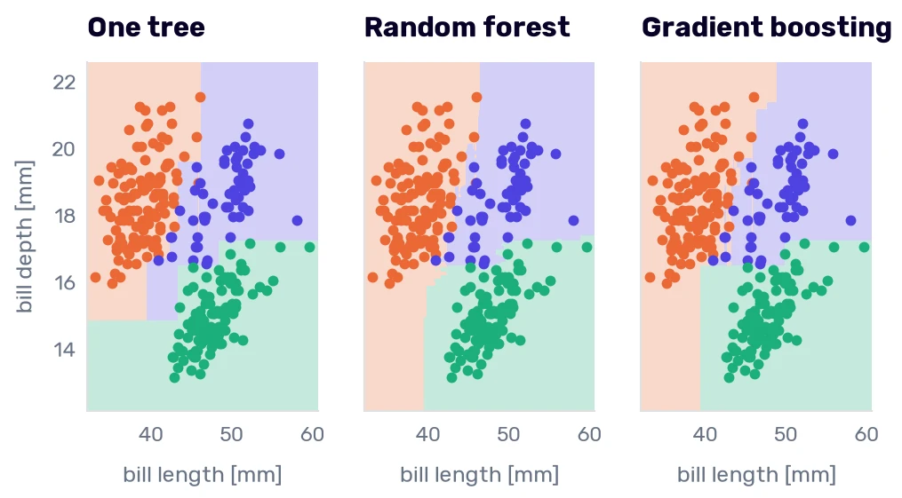
Every border runs parallel to an axis, because every question is about one column. A tree can only approximate the slanted border between the Adelies and the Chinstraps with steps. The forest and the boosting have more steps, and theirs are finer, but they are steps all the same. The logistic regression drew that border with one line.
Six models, a handful of penguins apart
models = {
    'nearest neighbors': species_knn,
    'logistic regression': logistic,
    'one tree': full_tree,
    'random forest': forest,
    'gradient boosting': boosting,
    'histogram gradient boosting': hist_boosting,
}

pd.DataFrame({name: fold_scores(model) for name, model in models.items()}).T.round(3)
| right | accuracy | balanced accuracy | log loss | |
|---|---|---|---|---|
| nearest neighbors | 269 | 0.985 | 0.975 | 0.033 |
| logistic regression | 269 | 0.985 | 0.979 | 0.06 |
| one tree | 264 | 0.967 | 0.957 | 1.188 |
| random forest | 266 | 0.974 | 0.966 | 0.083 |
| gradient boosting | 265 | 0.971 | 0.964 | 0.14 |
| histogram gradient boosting | 262 | 0.96 | 0.945 | 0.205 |
Seven penguins separate the best model from the worst. Rule 19 said to look at the folds before believing any of it:
fold_predictions = pd.DataFrame({
    name: cross_val_predict(model, train_df[numeric], species, cv=folds) for name, model in models.items()
}, index=train_df.index)

fold_number = pd.Series(0, index=train_df.index)
for number, (_, validation_rows) in enumerate(folds.split(train_df, species), start=1):
    fold_number.iloc[validation_rows] = number

right_per_fold = fold_predictions.eq(species, axis=0).groupby(fold_number).sum()
right_per_fold.assign(penguins=fold_number.value_counts().sort_index()).rename_axis('fold')
| fold | nearest neighbors | logistic regression | one tree | random forest | gradient boosting | histogram gradient boosting | penguins |
|---|---|---|---|---|---|---|---|
| 1 | 54 | 53 | 53 | 53 | 53 | 53 | 55 |
| 2 | 55 | 55 | 52 | 54 | 54 | 53 | 55 |
| 3 | 55 | 55 | 55 | 55 | 54 | 53 | 55 |
| 4 | 51 | 52 | 51 | 50 | 51 | 50 | 54 |
| 5 | 54 | 54 | 53 | 54 | 53 | 53 | 54 |
The nearest neighbors and the logistic regression trade one penguin in the first fold for one in the fourth, and that’s a tie by any reading. Neither is ever behind a tree model, and the forest is level with the logistic regression in three folds out of five. So the two simplest models are at least as good as the ensembles here. I can’t rank the ensembles among themselves on differences of one or two penguins per fold.
That isn’t how these comparisons usually end. On large tables with dozens of columns, missing values, and effects that depend on each other, gradient boosting usually comes out ahead. Our table has 273 rows and four columns, and the species nearly fall apart along straight lines, so a model that can only draw straight lines has all it needs, and the flexible ones have nothing extra to find, which we know only because we ran the simple models too.
The penguins they get wrong
Six models made 43 mistakes among them. How many different penguins is that?
wrong = fold_predictions.ne(species, axis=0)
wrong.any(axis=1).sum(), (wrong.sum(axis=1) >= 2).sum()
It returns (17, 8). Only 17 penguins were ever misclassified by anyone, and nine of them by a single model, which was a tree model every time. Eight were misclassified by at least two models:
missed = train_df.loc[wrong.sum(axis=1) >= 2, numeric + ['sex', 'species']].assign(models_wrong=wrong.sum(axis=1))
missed.sort_values('models_wrong', ascending=False)
| culmen_length_mm | culmen_depth_mm | flipper_length_mm | body_mass_g | sex | species | models_wrong | |
|---|---|---|---|---|---|---|---|
| 182 | 40.9 | 16.6 | 187 | 3200 | FEMALE | Chinstrap | 6 |
| 172 | 42.4 | 17.3 | 181 | 3600 | FEMALE | Chinstrap | 6 |
| 73 | 45.8 | 18.9 | 197 | 4150 | MALE | Adelie | 5 |
| 160 | 46 | 18.9 | 195 | 4150 | FEMALE | Chinstrap | 5 |
| 19 | 46 | 21.5 | 194 | 4200 | MALE | Adelie | 4 |
| 206 | 42.5 | 17.3 | 187 | 3350 | FEMALE | Chinstrap | 4 |
| 318 | 48.4 | 14.4 | 203 | 4625 | FEMALE | Gentoo | 2 |
| 157 | 45.2 | 17.8 | 198 | 3950 | FEMALE | Chinstrap | 2 |
Rows 182 and 172 are two Chinstraps that all six models call “Adelie”. Six models with nothing in common except the data agree on a wrong answer, so the answer comes from the data. Let’s put the eight on the chart:
species_regions(logistic, 'The penguins at least two models get wrong')
plt.scatter(missed[bill[0]], missed[bill[1]], s=160, facecolors='none', edgecolors='#080227', linewidths=1.5, label='wrong twice or more')
plt.legend()
plt.show()
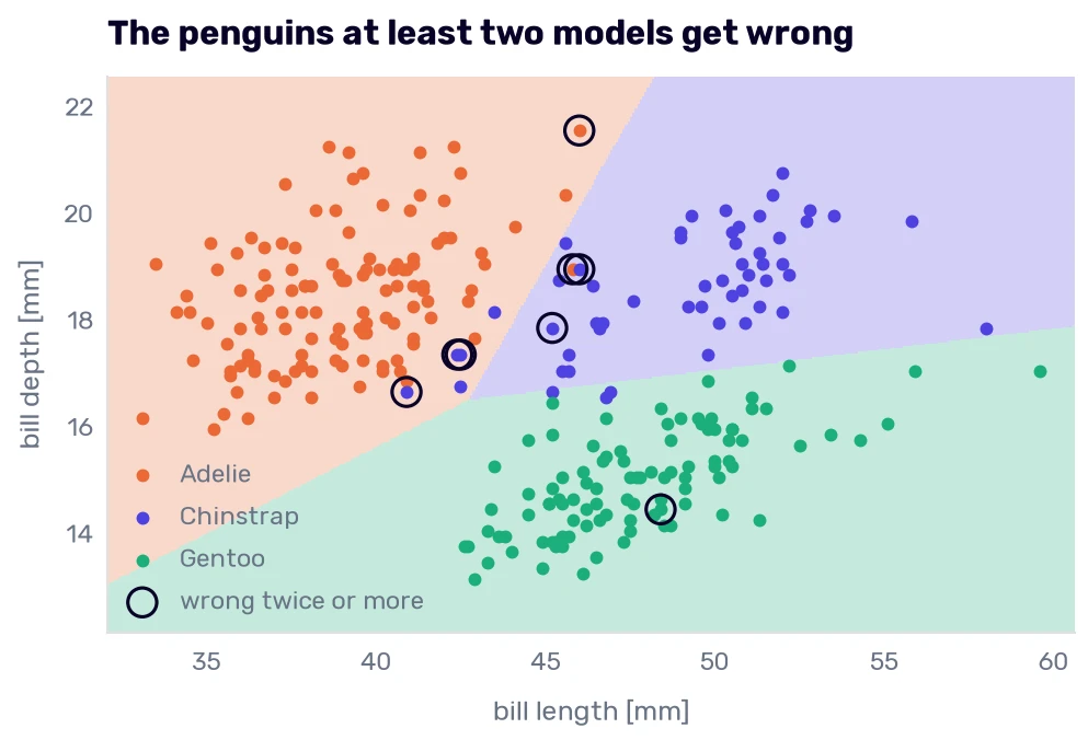
Seven of the eight sit along the border between the Adelies and the Chinstraps. (The eighth is a short-flippered Gentoo that only two tree models get wrong.)
Look at the sex column of the table. Five of the eight are Chinstrap females, and the two Adelies are males:
train_df.groupby(['species', 'sex'], observed=True)[numeric].mean().round(1)
| culmen_length_mm | culmen_depth_mm | flipper_length_mm | body_mass_g | |
|---|---|---|---|---|
| (‘Adelie’, ‘FEMALE’) | 37.3 | 17.7 | 187.7 | 3359.4 |
| (‘Adelie’, ‘MALE’) | 40.5 | 19.1 | 191.6 | 4057.1 |
| (‘Chinstrap’, ‘FEMALE’) | 46.7 | 17.7 | 192.4 | 3535.6 |
| (‘Chinstrap’, ‘MALE’) | 51.2 | 19.3 | 200.4 | 3970.5 |
| (‘Gentoo’, ‘FEMALE’) | 45.9 | 14.3 | 212.8 | 4676.5 |
| (‘Gentoo’, ‘MALE’) | 49.7 | 15.6 | 221.4 | 5508.3 |
Inside each species, the females have shorter bills than the males. So the birds closest to the border are the big-billed Adelies, who are males, and the small-billed Chinstraps, who are females. Row 172 has a bill of 42.4 mm. An average Chinstrap female has 46.7 mm, and an average Adelie male has 40.5 mm. Her bill is closer to an average Adelie male’s than to an average Chinstrap female’s. Her flipper (181 mm) is shorter than the average of any group in the table, and her bill depth and her mass would fit a female of either species. Nothing in the four numbers says “Chinstrap”. The two Adelies among the missed penguins, rows 73 and 19, have bills of 45.8 mm and 46.0 mm, and 46.0 mm is the longest Adelie bill in the training data.
Who are her neighbors? I take her out of the training data, the way the folds did, and ask:
others = train_df.drop(index=172)
knn_172 = clone(species_knn).fit(others[numeric], others['species'])
distances, positions = knn_172[-1].kneighbors(knn_172[0].transform(train_df.loc[[172], numeric]))
others.iloc[positions[0]][numeric + ['sex', 'species']].assign(distance=distances[0].round(2))
| culmen_length_mm | culmen_depth_mm | flipper_length_mm | body_mass_g | sex | species | distance | |
|---|---|---|---|---|---|---|---|
| 206 | 42.5 | 17.3 | 187 | 3350 | FEMALE | Chinstrap | 0.53 |
| 141 | 40.6 | 17.2 | 187 | 3475 | MALE | Adelie | 0.57 |
| 12 | 41.1 | 17.6 | 182 | 3200 | FEMALE | Adelie | 0.57 |
| 122 | 40.2 | 17 | 176 | 3450 | FEMALE | Adelie | 0.59 |
| 184 | 42.5 | 16.7 | 187 | 3350 | FEMALE | Chinstrap | 0.61 |
Three Adelies and two Chinstraps. The two Chinstraps are small-billed females like her, and one of them, row 206, is in the table of missed penguins herself. A small group of Chinstrap females lives inside the Adelie cloud, and each of them depends on the others for her vote.
At the end of The classification problem, I predicted that the hard penguins would be the Adelies and the Chinstraps with bills between 40.9 mm and 46.0 mm, and the heavy males of the two smaller species. The first half held: that range contains 43 training penguins, and all four mistakes of the logistic regression and all four of the nearest neighbors are among them. Each model gets the other 39 right, because the other three columns help. The second half was wrong. Neither of the two best models ever confused anything with a Gentoo, since the Gentoos differ in three columns at once.
What would fix rows 182 and 172? A seventh model wouldn’t. They sit among Adelies in every column we have, and Rule 16 said that no rearrangement of four measurements will add what the measurements don’t hold. A person standing in front of the bird would look for the black line under the chin. The data has two more columns we haven’t used, and one of them, the sex, is exactly what separates “a big Adelie” from “a small Chinstrap” in the table of averages. We try both in What the island and the sex are worth.
A second opinion
There is something we can do without new columns. The models that give probabilities tell us how sure they are. Is the logistic regression less sure about the penguins it gets wrong?
shares = cross_val_predict(logistic, train_df[numeric], species, cv=folds, method='predict_proba')
answers = pd.DataFrame({
    'species': species,
    'predicted': logistic[-1].classes_[shares.argmax(axis=1)],
    'probability': shares.max(axis=1),
}, index=train_df.index)
answers['wrong'] = answers['species'] != answers['predicted']
answers[answers['wrong']].round(3)
| species | predicted | probability | wrong | |
|---|---|---|---|---|
| 206 | Chinstrap | Adelie | 0.559 | True |
| 73 | Adelie | Chinstrap | 0.558 | True |
| 182 | Chinstrap | Adelie | 0.692 | True |
| 172 | Chinstrap | Adelie | 0.752 | True |
It is. The four wrong answers came with probabilities between 0.56 and 0.75, and the model gives 213 of the 273 penguins more than 0.95. Suppose we accept an answer only above some limit and send the other penguins to somebody who can look at the chin:
rows = []
for limit in [0.6, 0.7, 0.8, 0.9, 0.95]:
    unsure = answers['probability'] < limit
    rows.append({
        'limit': limit,
        'sent for a second opinion': unsure.sum(),
        'mistakes among them': answers.loc[unsure, 'wrong'].sum(),
        'answers kept': (~unsure).sum(),
        'mistakes kept': answers.loc[~unsure, 'wrong'].sum(),
    })

pd.DataFrame(rows).set_index('limit')
| limit | sent for a second opinion | mistakes among them | answers kept | mistakes kept |
|---|---|---|---|---|
| 0.6 | 5 | 2 | 268 | 2 |
| 0.7 | 9 | 3 | 264 | 1 |
| 0.8 | 14 | 4 | 259 | 0 |
| 0.9 | 34 | 4 | 239 | 0 |
| 0.95 | 60 | 4 | 213 | 0 |
With a limit of 0.8, 14 penguins need a second opinion, all four mistakes are among them, and the 259 answers we keep are all correct. In Scores and thresholds, the sex classifier sent 41 penguins to the lab for the same reason.
Real systems are built this way. I heard about one when I worked on a website with hotel offers. We were discussing how to check that a photo in a hotel’s profile is in the right category (a photo filed under “restaurant” should show a restaurant, and it’s often a beach) and that it follows the guidelines (no people in the pictures, for example). Our product owner had worked at a marketplace before. There, the pictures posted with the offers had to be censored, because people were, as she put it, “very creative.” Somebody had posted a photo of a corpse as a product picture. What the marketplace built was a setup in layers: a cheap model settles the pictures it’s sure about and passes the rest on to a bigger, more expensive one. She also told me that checking the content in the “adult” category was the most mentally taxing work there, and that people asked to move to another project after a few months, which is one more reason to let a model settle every picture it can.
Don’t copy the table above into a design document yet.
I picked the limit of 0.8 after seeing where the mistakes were, on the same folds. It’s the best of five tries, and it fits these 273 penguins a little too well. In a real project, the limit is a setting like any other and gets chosen on validation data, as we said about thresholds.
The probabilities have to mean something. The logistic regression is trained on the log loss, which rewards honest probabilities, so its 0.56 is a real doubt. The fully grown tree said 1.0 about all nine of its mistakes. A limit on its probabilities would send nobody for a second opinion.
And a high probability only says that a row is far from the border, on the side of one class. It doesn’t say the row looks like anything the model has seen. Hand our model an Emperor penguin, 120 cm tall and 30 kg, and it will answer “Gentoo” with a probability of nearly 1, because for a linear score, more mass and a longer flipper are simply more Gentoo. A check on the model’s confidence catches the rows near the border. For rows unlike anything in the training data, you need a separate check on the inputs, like the range checks in the data drift section.
What the island and the sex are worth
I promised to train the models with and without the two columns we left out. First, the island, one-hot encoded next to the scaled measurements:
from sklearn.preprocessing import OneHotEncoder

with_island = make_pipeline(
    ColumnTransformer([('numeric', StandardScaler(), numeric), ('island', OneHotEncoder(), ['island'])]),
    LogisticRegression(),
)
pd.DataFrame({'with the island': fold_scores(with_island, numeric + ['island'])}).T.round(3)
| right | accuracy | balanced accuracy | log loss | |
|---|---|---|---|---|
| with the island | 271 | 0.993 | 0.988 | 0.041 |
271, two more penguins. The Adelie in row 73 lives on Torgersen, where there are only Adelies, and one of the Chinstraps is saved by living on Dream. Rows 182 and 172 are still wrong. They live on Dream too, but so do 44 Adelies.
I’m still leaving the island out. It describes where the researchers went. Two penguins on the folds are within what we called a tie when we compared the six models, and a model without the island would also work on a fourth one.
The sex takes more care. We worked out that a new penguin arrives without a DNA test, so the model will get a guess from the fill_sex pipeline. The folds have to do the same: train on the real sex, then blank it in the validation part and let the imputer fill it. cross_val_predict() can’t blank a column, so the loop is written out:
def sex_folds(model, blank):
    columns = numeric + ['sex']
    predicted = pd.Series(index=train_df.index, dtype=object)
    for train_rows, validation_rows in folds.split(train_df, species):
        fitted = clone(model).fit(train_df[columns].iloc[train_rows], species.iloc[train_rows])
        validation = train_df[columns].iloc[validation_rows].copy()
        if blank:
            validation['sex'] = pd.Series(np.nan, index=validation.index, dtype=object)
        predicted.iloc[validation_rows] = fitted.predict(validation)
    return (predicted == species).sum()

pd.DataFrame({
    name: {
        'without the sex': fold_scores(make_pipeline(StandardScaler(), model))['right'],
        'the real sex in validation': sex_folds(make_pipeline(fill_sex, model), blank=False),
        'the sex blanked and imputed': sex_folds(make_pipeline(fill_sex, model), blank=True),
    }
    for name, model in [('logistic regression', LogisticRegression()), ('nearest neighbors', KNeighborsClassifier(n_neighbors=5))]
}).T
| without the sex | the real sex in validation | the sex blanked and imputed | |
|---|---|---|---|
| logistic regression | 269 | 270 | 267 |
| nearest neighbors | 269 | 270 | 269 |
With the real sex, both models gain one penguin. With the sex blanked and imputed, which is what a new penguin would get, the nearest neighbors are back at 269, and the logistic regression is at 267. A difference of one or two penguins was a tie when we compared the six models, and the same standard applies here. The three columns can’t be told apart.
So the counts give no reason to add the sex, and there is a reason to leave it out that doesn’t depend on them. In use, the column holds a guess made from the same four measurements the model already has, so it can’t tell the model anything new. In What a new penguin gets, I said that folds with the real sex would overstate what the column is worth. The table points that way, by one to three penguins, which is too few to call it confirmed. The species model gets the four measurements and nothing else.
One promise is left. In What a new penguin gets, I claimed that mates on both sides of a fold don’t leak anything about the species. I also said that splitting the folds by nest would show whether I was right. StratifiedGroupKFold keeps the two birds of a nest in the same fold:
from sklearn.model_selection import StratifiedGroupKFold

nests = raw.loc[train_df.index, 'nest']
nest_folds = StratifiedGroupKFold(n_splits=5, shuffle=True, random_state=42)

pd.Series({
    name: (cross_val_predict(model, train_df[numeric], species, cv=nest_folds, groups=nests) == species).sum()
    for name, model in [('nearest neighbors', species_knn), ('logistic regression', logistic), ('random forest', forest)]
}, name='right, folds split by nest')
| right, folds split by nest | |
|---|---|
| nearest neighbors | 269 |
| logistic regression | 268 |
| random forest | 268 |
The ordinary folds gave 269, 269, and 266. Of the 109 nests with both adults in the training data, they had put the two birds of 96 into different folds. With every pair kept together, the counts move by one or two penguins in both directions, which is what a different shuffle does anyway. I see no sign of a leak, so the ordinary folds stay.
One look at the test set
We have a species model that beats both baselines by a wide margin on the folds, so this chapter gets its look at the test set (Rule 14).
The model is the logistic regression on the four scaled measurements, with scikit-learn’s default C. It ties with the nearest neighbors on the folds, and I take it because it’s 15 numbers and a scaler where the neighbors have to carry all 273 training penguins around, and because its probabilities told us which answers to doubt.
The expectation: 269 of 273 on the folds is one mistake in every 68 penguins, and the test set has 69. Rule 25 told us to know the counts, and one penguin is 1.4 percentage points here, so anything from 67 to 69 correct answers would be unsurprising. The mistakes, if any, should be Chinstraps and Adelies with bills of 41 mm to 46 mm. The baselines on the same 69 penguins are 30 for the dummy and whatever the island rule gets.
logistic.fit(train_df[numeric], species)
test_predicted = logistic.predict(test_df[numeric])

by_island = test_df['island'].map(island_rule)
(by_island == test_df['species']).sum(), balanced_accuracy_score(test_df['species'], by_island)
(np.int64(48), 0.7666666666666666)
confusion_matrix(test_df['species'], test_predicted)
array([[30,  0,  0],
       [ 0, 14,  0],
       [ 0,  0, 25]])
The island rule gets 48 of 69 (77% balanced). The logistic regression gets 69 of 69.
A perfect score deserves the same suspicion as a bad one, so let’s see what it’s made of. If the model’s true rate is the 98.5% from the folds, the chance of 69 correct answers in a row is 0.985 to the power of 69, which is 35%. A model exactly as good as the folds say would produce this result every third time. The model didn’t get better between the folds and the test set. The test set happened to contain no penguin like row 172.
It came close, though:
test_shares = logistic.predict_proba(test_df[numeric]).max(axis=1)
test_df[test_shares < 0.8].assign(predicted=test_predicted[test_shares < 0.8], probability=test_shares[test_shares < 0.8].round(3))
| species | island | culmen_length_mm | culmen_depth_mm | flipper_length_mm | body_mass_g | sex | predicted | probability | |
|---|---|---|---|---|---|---|---|---|---|
| 37 | Adelie | Dream | 42.2 | 18.5 | 180 | 3550 | FEMALE | Adelie | 0.794 |
| 129 | Adelie | Torgersen | 44.1 | 18 | 210 | 4000 | MALE | Adelie | 0.512 |
Two test penguins fall under the limit of 0.8 from A second opinion. Row 129, an Adelie male with a bill of 44.1 mm, got the right answer with a probability of 0.51. With one more millimeter of bill, the headline would be 68 of 69.
So the number I would report for this model is the one from the folds: about 269 of 273, with the mistakes among the small-billed Chinstrap females and the big-billed Adelie males. The test set didn’t contradict it, which is all that 69 penguins can do.
Look at who pays for the mistakes, though. On the folds, the Adelies had a recall of 99% and the Gentoos of 100%. The Chinstraps had 94% (51 of 54), and they are the species we have the fewest of: 54 penguins against 121 Adelies. It’s tempting to blame the class sizes. Scikit-learn can make every species count the same during training, however many penguins it has:
balanced = make_pipeline(StandardScaler(), LogisticRegression(class_weight='balanced'))
balanced_predicted = cross_val_predict(balanced, train_df[numeric], species, cv=folds)
(balanced_predicted == species).sum(), train_df.index[balanced_predicted != species].tolist()
(np.int64(270), [73, 182, 172])
Row 206 comes back, and one penguin is a tie. Rows 182 and 172 stay wrong. Their measurements overlap with the Adelies’, and no weighting changes the measurements. Our classes are only mildly unequal. In the next chapter, I will show you how to deal with imbalanced datasets (we will pretend that the penguins are such a case).