
Classification predicts a category. In the regression chapters, the answer was a number, and a prediction 2 mpg away from the truth was better than one 10 mpg away. A category has no “closer,” because the penguin in front of you either is a Gentoo or it isn’t. Wait, why a penguin?
In the classification part of the book, we use the “Palmer Penguins” dataset: 344 penguins of three species, measured on three islands near Palmer Station in Antarctica.1 Given a penguin’s measurements, we will predict its species. In 2020, the data was repackaged as an alternative to iris, the flower dataset that opens every classification tutorial. Unlike iris, it has problems to find, and the fourth row below is the first of them.
Is that a useful model? For any real-world purpose, no. Anyone close enough to measure a penguin’s bill can see its species: a Chinstrap has a thin black line under its chin, and a Gentoo has an orange bill. I said the same about the cars (useless for any real-world prediction, fine for teaching), and the penguins are here for the same reason. A small table with real flaws is a good place to practice what you will later have to do to your own model.
import matplotlib.pyplot as plt
import numpy as np
import pandas as pd
from sklearn.datasets import fetch_openml

df = fetch_openml(data_id=42585, as_frame=True).frame
df.head()
| species | island | culmen_length_mm | culmen_depth_mm | flipper_length_mm | body_mass_g | sex |
|---|---|---|---|---|---|---|
| Adelie | Torgersen | 39.1 | 18.7 | 181 | 3750 | MALE |
| Adelie | Torgersen | 39.5 | 17.4 | 186 | 3800 | FEMALE |
| Adelie | Torgersen | 40.3 | 18 | 195 | 3250 | FEMALE |
| Adelie | Torgersen | nan | nan | nan | nan | nan |
| Adelie | Torgersen | 36.7 | 19.3 | 193 | 3450 | FEMALE |
The documentation I linked describes a different version of the data. Again. It calls the two bill columns bill_length_mm and bill_depth_mm, writes the sex in lowercase, and has an eighth column with the year of the measurement. The version we downloaded says “culmen”, shouts MALE and FEMALE, and has no year. (The missing year matters in a minute, when we split the data.)
-
species: the target variable. Adelie, Chinstrap, or Gentoo -
island: where the penguin was measured. Biscoe, Dream, or Torgersen -
culmen_length_mm: the culmen is the upper ridge of the bill, and its length runs from the base of the bill to the tip. I will call it the bill length, like the documentation does -
culmen_depth_mm: how tall the bill is, from the top to the bottom. The bill depth from now on -
flipper_length_mm: the length of the flipper in millimeters -
body_mass_g: the body mass in grams -
sex: MALE or FEMALE
Rule 1 hasn’t changed, so we check before we believe any of it. df.shape returns (344, 7), which matches the 344 penguins the documentation promises. df.dtypes says the four measurements are float64 and the other three columns are category, the pandas type for a column with a fixed set of text values. So far, the file loaded the way it should.
How many penguins of each species do we have?
df['species'].value_counts()
| species | count |
|---|---|
| Adelie | 152 |
| Gentoo | 124 |
| Chinstrap | 68 |
A model that answers “Adelie” for every penguin is right 152 times out of 344, which is 44%. That’s the dummy model Rule 10 asks for, and every classifier in the next chapters has to beat it. We also have fewer than half as many Chinstraps as Adelies, which will get in the way as soon as we split the data.
Splitting the penguins
Rule 9 says the split comes from the question we’re answering, so let’s state the question: given the measurements of a penguin from one of these three islands, which species is it? The cars were split by year, because the model had to predict cars built after the ones it learned from. The penguins were measured over three summers, but our version of the file has no year, so we couldn’t hold out the last summer even if we wanted to.
A random split answers exactly the question we stated. The test penguins will be more like the birds from the same colonies and the same summers, so the test score won’t tell us how the model does on penguins measured anywhere else. With that written down, a random split is fine here, as long as we avoid two traps.
The first trap is the order of the rows. The file is sorted by species: rows 0-151 are Adelie, 152-219 are Chinstrap, and 220-343 are Gentoo. Here is what the last 20% of the file looks like:
df['species'].tail(69).value_counts()
| species | count |
|---|---|
| Gentoo | 69 |
| Adelie | 0 |
| Chinstrap | 0 |
If we took the end of the file as the test set, we would test on Gentoos only, and every model that says “Gentoo” a lot would look brilliant. So the split has to shuffle the rows.
The second trap is the 68 Chinstraps. A shuffle could put 9 of them in the test set, or 19, by luck alone. A stratified split shuffles within each species, so both datasets get the three species in the same proportions:
from sklearn.model_selection import train_test_split

train_df, test_df = train_test_split(df, test_size=0.2, stratify=df['species'], random_state=42)
pd.DataFrame({'train': train_df['species'].value_counts(), 'test': test_df['species'].value_counts()})
| species | train | test |
|---|---|---|
| Adelie | 122 | 30 |
| Gentoo | 99 | 25 |
| Chinstrap | 54 | 14 |
With the cars, we explored every row before the split, including the rows that later became the test set. This time, we split first, so everything below comes from the 275 training penguins, and the 69 test penguins stay unseen. (No model gets trained in this chapter, so we don’t spend a look at the test set either.)
What is missing
The fourth row of the file was almost empty, so let’s count:
train_df.isna().sum()
| 0 | |
|---|---|
| species | 0 |
| island | 0 |
| culmen_length_mm | 2 |
| culmen_depth_mm | 2 |
| flipper_length_mm | 2 |
| body_mass_g | 2 |
| sex | 10 |
train_df[train_df.isna().any(axis=1)].sort_index()
| species | island | culmen_length_mm | culmen_depth_mm | flipper_length_mm | body_mass_g | sex | |
|---|---|---|---|---|---|---|---|
| 3 | Adelie | Torgersen | nan | nan | nan | nan | nan |
| 8 | Adelie | Torgersen | 34.1 | 18.1 | 193 | 3475 | nan |
| 9 | Adelie | Torgersen | 42 | 20.2 | 190 | 4250 | nan |
| 10 | Adelie | Torgersen | 37.8 | 17.1 | 186 | 3300 | nan |
| 11 | Adelie | Torgersen | 37.8 | 17.3 | 180 | 3700 | nan |
| 47 | Adelie | Dream | 37.5 | 18.9 | 179 | 2975 | nan |
| 246 | Gentoo | Biscoe | 44.5 | 14.3 | 216 | 4100 | nan |
| 286 | Gentoo | Biscoe | 46.2 | 14.4 | 214 | 4650 | nan |
| 324 | Gentoo | Biscoe | 47.3 | 13.8 | 216 | 4725 | nan |
| 339 | Gentoo | Biscoe | nan | nan | nan | nan | nan |
Two penguins (rows 3 and 339) have a species, an island, and nothing else. The other eight were measured, but nobody recorded their sex. Is that all of it? Rule 3 says a check that passes rules out only the errors you thought to look for, and isna() looks for one kind of missing value. Let’s look at what the sex column contains:
train_df['sex'].value_counts(dropna=False)
| sex | count |
|---|---|
| MALE | 134 |
| FEMALE | 130 |
| nan | 10 |
| _ | 1 |
One Gentoo (row 336) has the sex “_”. It’s the sentinel value I complained about in Examining the data: a missing value written down as something other than a null. isna() found 10 penguins without a sex, and there are 11.
We will deal with all of them in the next chapter. With the cars, I dropped the six incomplete rows and admitted it wasn’t the best we could do. The penguins give us more to work with. Until then, every chart below leaves out the values a penguin doesn’t have.
The duplicates check from Examining the data passes: train_df.duplicated().sum() returns 0, and no two measured penguins share all four measurements. Rule 8 asks for more than a string comparison, though. The paper behind the dataset says the researchers captured both adults at each nest, and the file seems to keep them together. When I pair up consecutive rows, 163 of the 172 pairs hold one male and one female.
Our shuffle put the two birds of 55 of those 172 pairs on different sides of the split. I don’t think it leaks anything. Mates are two different animals with their own measurements, and all the file says they share is a species and an island. Still, the rows aren’t as independent as a random split assumes, and if we ever used a feature that describes the nest, we would have to split by pair.
One more boring check before the charts. Here is train_df.describe():
| culmen_length_mm | culmen_depth_mm | flipper_length_mm | body_mass_g | |
|---|---|---|---|---|
| count | 273 | 273 | 273 | 273 |
| mean | 44.0678 | 17.1707 | 200.846 | 4211.26 |
| std | 5.49999 | 2.01453 | 13.9644 | 805.746 |
| min | 33.1 | 13.1 | 172 | 2700 |
| 25% | 39.5 | 15.5 | 190 | 3550 |
| 50% | 44.9 | 17.3 | 197 | 4050 |
| 75% | 48.7 | 18.8 | 213 | 4775 |
| max | 59.6 | 21.5 | 231 | 6300 |
Nothing is zero or negative. The lightest penguin weighs 2700 g and the heaviest 6300 g, so nobody mixed grams with kilograms. The flippers run from 172 mm to 231 mm, which rules out a row typed in centimeters.
The flipper has two peaks
In Examining the data, we expected the displacement histogram to have several peaks, one per engine family. Three species in one table should do the same thing to a body measurement. Here is the flipper length, first for all the training penguins and then with the bars colored by species:
SPECIES_COLORS = {'Adelie': '#eb6834', 'Chinstrap': '#4d41e0', 'Gentoo': '#1baf7a'}

bins = range(170, 236, 3)
fig, (top, bottom) = plt.subplots(2, 1, sharex=True, figsize=(7.6, 6))

top.hist(train_df['flipper_length_mm'].dropna(), bins=bins, color='#687385')
top.set_title('Flipper length, all training penguins', loc='left')
top.set_ylabel('penguins')

flippers = [train_df.loc[train_df['species'] == species, 'flipper_length_mm'].dropna() for species in SPECIES_COLORS]
bottom.hist(flippers, bins=bins, stacked=True, color=list(SPECIES_COLORS.values()), label=list(SPECIES_COLORS))
bottom.set_title('The same histogram, colored by species', loc='left')
bottom.set_xlabel('flipper length [mm]')
bottom.set_ylabel('penguins')
bottom.legend()

plt.tight_layout()
plt.show()
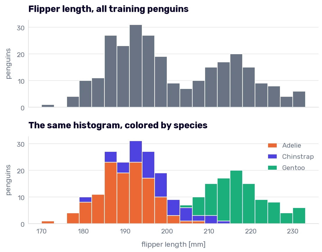
Three species, and only two peaks, with a dip around 205 mm between them. The colors explain why. The right peak belongs to the Gentoos (the shortest Gentoo flipper in the training data is 203 mm, and only 13 of the 175 measured Adelies and Chinstraps reach that length), and the left peak is the other two species stacked on top of each other. One column gets us most of the way to the Gentoos, and it doesn’t help at all with the other two.
Bigger penguins
Let’s add a second measurement. I’ll draw several of these charts, so the drawing goes into a function:
def species_scatter(x, y, x_label, y_label, title):
    for species, color in SPECIES_COLORS.items():
        rows = train_df[train_df['species'] == species]
        plt.scatter(rows[x], rows[y], color=color, label=species, alpha=0.8)
    plt.title(title, loc='left')
    plt.xlabel(x_label)
    plt.ylabel(y_label)
    plt.legend()

species_scatter('flipper_length_mm', 'body_mass_g', 'flipper length [mm]', 'body mass [g]', 'Body mass and flipper length')
plt.show()
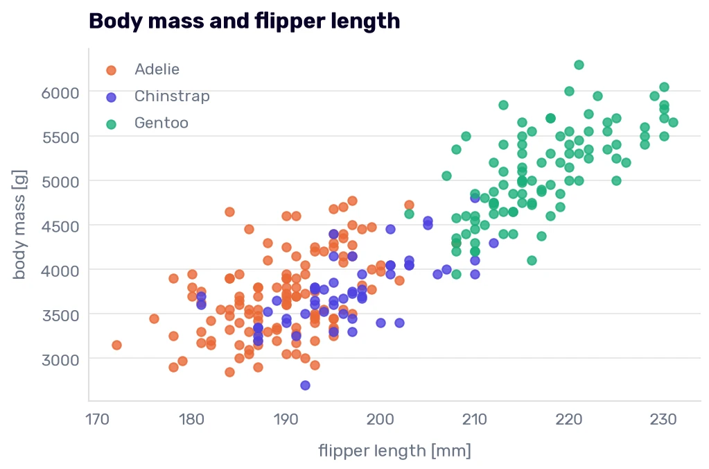
The Gentoos sit in the upper-right corner, with longer flippers and more weight, because they are bigger birds. I took the photo below at Chimelong Ocean Kingdom in Zhuhai, China. The wall gives a Gentoo 76 cm of height, a good step below the King and the Emperor.
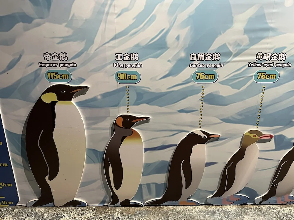
Adelie and Chinstrap were in a more crowded section of the wall, so I didn’t take a picture, and our dataset has no height column anyway. It has the mass:
numeric = ['culmen_length_mm', 'culmen_depth_mm', 'flipper_length_mm', 'body_mass_g']
train_df.groupby('species', observed=True)[numeric].mean().round(1)
| species | culmen_length_mm | culmen_depth_mm | flipper_length_mm | body_mass_g |
|---|---|---|---|---|
| Adelie | 38.9 | 18.4 | 189.7 | 3705.4 |
| Chinstrap | 49 | 18.5 | 196.6 | 3761.1 |
| Gentoo | 47.7 | 14.9 | 217 | 5083.9 |
An average Gentoo weighs 5084 g, over 1.3 kg more than an average Adelie or Chinstrap. The mass separates them worse than the flipper does, though. The lightest Gentoo weighs 3950 g, and 55 of the other penguins weigh at least that much (remember, only 13 had flippers as long as the shortest Gentoo’s).
What about the orange and the indigo dots? The Adelies and the Chinstraps differ by 56 g and 7 mm on average, and in this chart they are one cloud. If these two columns were all we had, the model would have to guess between them.
The same table says where to look next. The Adelie’s bill is 38.9 mm long, and the Chinstrap’s is 49.0 mm. Here is the bill length against the flipper length (the documentation draws the same chart):
species_scatter('flipper_length_mm', 'culmen_length_mm', 'flipper length [mm]', 'bill length [mm]', 'Bill length and flipper length')
plt.show()
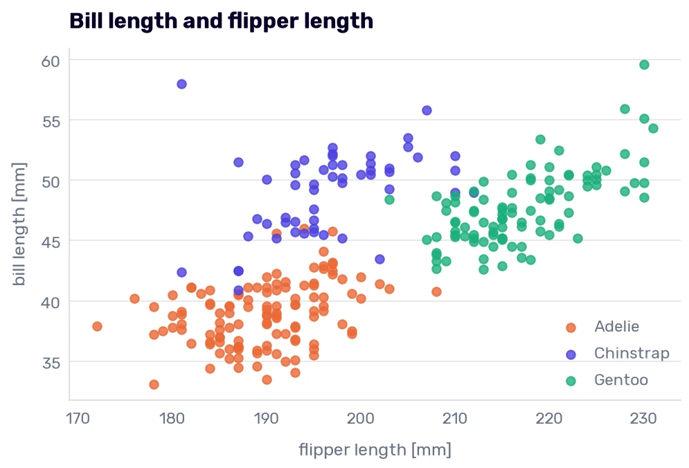
Three clouds, finally. The flipper separates the Gentoos from the rest, and the bill length separates the Adelies from the Chinstraps, although those two still overlap. The shortest Chinstrap bill is 40.9 mm, and 30 Adelies have a bill at least that long. Going the other way, 13 Chinstraps have a bill no longer than the longest Adelie’s (46.0 mm). Those are the penguins a classifier will get wrong first, and Chinstrap is the species we have the fewest of.
A correlation that points the wrong way
In Improving the model, we read a correlation matrix to find columns that carry the same information. Here is the penguin version:
train_df[numeric].corr().round(2)
| culmen_length_mm | culmen_depth_mm | flipper_length_mm | body_mass_g | |
|---|---|---|---|---|
| culmen_length_mm | 1 | -0.24 | 0.68 | 0.6 |
| culmen_depth_mm | -0.24 | 1 | -0.59 | -0.48 |
| flipper_length_mm | 0.68 | -0.59 | 1 | 0.87 |
| body_mass_g | 0.6 | -0.48 | 0.87 | 1 |
Flipper length and body mass correlate at 0.87, which we have already seen in the chart. The odd numbers are in the bill-depth row. According to this table, a longer bill is a shallower bill (−0.24), and a heavier penguin has a shallower bill too (−0.48). That would be a strange way to build a bird. Let’s draw the first of the two, with a trend line for all the penguins and one for each species:
def trend_line(rows, color, label=None, **style):
    rows = rows.dropna(subset=['culmen_length_mm', 'culmen_depth_mm'])
    slope, intercept = np.polyfit(rows['culmen_length_mm'], rows['culmen_depth_mm'], 1)
    ends = np.array([rows['culmen_length_mm'].min(), rows['culmen_length_mm'].max()])
    plt.plot(ends, slope * ends + intercept, color=color, label=label, **style)

species_scatter('culmen_length_mm', 'culmen_depth_mm', 'bill length [mm]', 'bill depth [mm]', 'Bill depth and bill length')
for species, color in SPECIES_COLORS.items():
    trend_line(train_df[train_df['species'] == species], color)
trend_line(train_df, '#080227', label='all penguins', linestyle='--')
plt.legend()
plt.show()
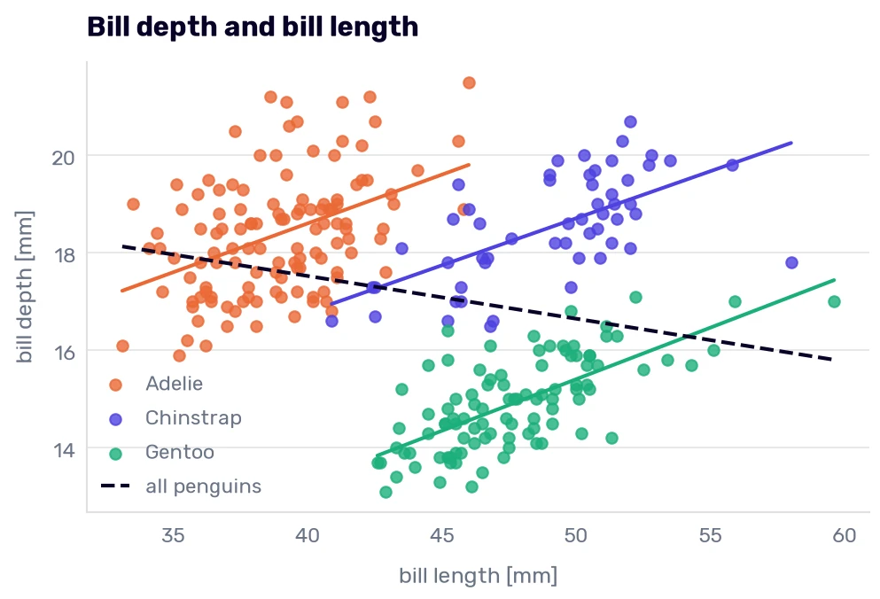
The dashed line falls while all three colored lines rise. Inside each species, the correlation between bill length and bill depth is positive: 0.43 for Adelie, 0.62 for Chinstrap, and 0.68 for Gentoo. A longer bill is a deeper bill, as you would expect from a bigger bird of the same kind.
The negative number comes from mixing the species. Gentoos have long and shallow bills (47.7 mm by 14.9 mm on average), and Adelies have short and deep ones (38.9 mm by 18.4 mm). When both clouds land in one table, the line through them runs from the upper left to the lower right, although no penguin’s bill works like that. Statisticians call it Simpson’s paradox. The correlation matrix can’t show it, because it never sees the species column.
We have seen a sign flip like this one before. In Reading the coefficients, every extra second of acceleration added 1.00 mpg when the column was fitted alone and took 0.15 mpg away when it was fitted together with the other five columns. It’s the same thing happening.
For our classifier, the chart is good news, because bill length and bill depth together put the three species in three clouds, which neither column does alone.
Males and females
There is one more group hiding in every chart above:
known_sex = train_df[train_df['sex'].isin(['MALE', 'FEMALE'])]
known_sex.pivot_table(index='species', columns='sex', values='body_mass_g', aggfunc='mean', observed=True).round(0)
| species | FEMALE | MALE |
|---|---|---|
| Adelie | 3365 | 4060 |
| Chinstrap | 3536 | 3971 |
| Gentoo | 4684 | 5508 |
In every species, the males are heavier, by 435 to 824 g. An average male Adelie (4060 g) is much closer to an average female Gentoo (4684 g) than the two species averages suggested. Of the 55 Adelies and Chinstraps that weigh as much as the lightest Gentoo, 52 are males.
So the sex would help the model, but where does that column come from? You can’t tell a male penguin from a female by looking, so the researchers took blood samples and determined the sex with a DNA test. Whoever uses our model with a ruler and a scale won’t have a lab result. If nobody can provide a feature at prediction time, the model can’t use it, and we will have to remember that when we choose the features.
Three islands
The last column we haven’t looked at is the island:
islands = pd.crosstab(train_df['species'], train_df['island'])
islands
| species | Biscoe | Dream | Torgersen |
|---|---|---|---|
| Adelie | 35 | 44 | 43 |
| Chinstrap | 0 | 54 | 0 |
| Gentoo | 99 | 0 | 0 |
Every Chinstrap was measured on Dream, every Gentoo on Biscoe, and Torgersen has nothing but Adelies. Where are those islands?
import folium

# Coordinates from Gorman, Williams, and Fraser (2014)
ISLANDS = {'Biscoe': (-64.800, -63.767), 'Dream': (-64.717, -64.217), 'Torgersen': (-64.767, -64.067)}
PALMER_STATION = (-64.774, -64.053)

island_map = folium.Map(location=(-64.76, -64.0), zoom_start=11, control_scale=True)
for island, location in ISLANDS.items():
    species_here = ', '.join(islands.index[islands[island] > 0])
    folium.Marker(location, tooltip=folium.Tooltip(f'{island}: {species_here}', permanent=True)).add_to(island_map)
# The research station is 1 km from Torgersen, so it gets a small red dot and a label on the left
folium.CircleMarker(PALMER_STATION, radius=6, color='#fc7272', fill=True, fill_opacity=1,
                    tooltip=folium.Tooltip('Palmer Station', permanent=True, direction='left')).add_to(island_map)
island_map.save('penguin_islands.html')
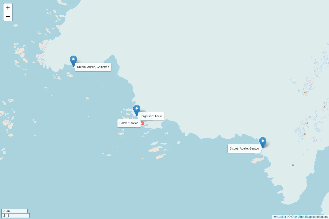
The three sites are 9 to 23 km from each other, all of them within 15 km of Palmer Station. (My first version of this map had Biscoe 107 km to the southwest. I had taken the coordinates of the Biscoe Islands, which is a different place with almost the same name. The coordinates above come from the paper by Gorman, Williams, and Fraser. Rule 4, on myself.)
What would a model do with the island column? Suppose it looks at nothing else and answers “Gentoo” on Biscoe, “Chinstrap” on Dream, and “Adelie” on Torgersen. It gets 196 of the 275 training penguins right, which is 71% without measuring a single bird (always saying “Adelie” got us 44%).
That 71% describes where the researchers found the colonies around one research station, and a model can score it without knowing what a Gentoo looks like. A model that learned “Biscoe means Gentoo” works until somebody measures penguins on a fourth island, and then it’s the brewery camera on the day the bottles changed color. Our test set can’t warn us about that. Its penguins come from the same three islands, where the same rule keeps working. I’m leaving the island out of the features for now anyway, so the first models have to learn the birds. We can add it back later and see what it’s worth.
One more thing about penguins that no column records. The second photo comes from the same park:
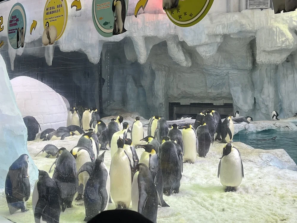
These are Emperor penguins, which aren’t in our dataset, but look at the ice they stand on. It smelled like a urinal at a train station in a post-Soviet country. The researchers spent three summers in colonies like this one to collect the 344 rows we downloaded for free.
Before the first model
The measurements are on very different scales: the body mass runs from 2700 g to 6300 g with a standard deviation of 806 g, and the bill depth from 13.1 mm to 21.5 mm with a standard deviation of 2.0 mm. We know from The nearest cars that a column 400 times wider than another decides the distance almost alone. With the cars, that column was the weight, the best one we had. Here, it would be the body mass, which can’t tell an Adelie from a Chinstrap. Every penguin model that measures distances or penalizes coefficients will get a scaler.
We also know which penguins will be hard: the Adelies and Chinstraps with bills between 40.9 mm and 46.0 mm, and the heavy males of the two smaller species. When a classifier starts making mistakes, we will open those rows first.
Before that, we have 11 training penguins with something missing, and the next chapter has to decide what to do with them.
-
The data was collected by Dr. Kristen Gorman and the Palmer Station Long Term Ecological Research program during three Antarctic summers, from 2007/08 to 2009/10. It was published with Gorman, Williams, and Fraser (2014), which is also where the island coordinates and the description of the sex test come from. ↩