
Imbalanced datasets ended with a model that was missing columns. Without the bill, no resampler could find the Chinstraps, and I promised to look at the columns again and ask which of them a model needs.
Feature selection usually means the opposite problem. You have 200 columns, most of them useless, and you want the 15 that matter. The penguins have four, and I can’t teach you to choose from four. So this chapter goes both ways. First, we look for more columns, and then we learn how to throw columns away, which includes most of the ones we just found.
Every subset of four columns
Four columns have one advantage. They can be combined in only 15 ways, so we can train a model on every combination and skip the clever methods:
from itertools import combinations

def right(model, table):
    return int((cross_val_predict(model, table, species, cv=folds) == species).sum())

short = {'culmen_length_mm': 'bill length', 'culmen_depth_mm': 'bill depth', 'flipper_length_mm': 'flipper', 'body_mass_g': 'mass'}
subsets = [list(columns) for size in range(1, 5) for columns in combinations(numeric, size)]

pd.DataFrame({
    'logistic regression': [right(logistic, train_df[columns]) for columns in subsets],
    'nearest neighbors': [right(species_knn, train_df[columns]) for columns in subsets],
}, index=[', '.join(short[column] for column in columns) for columns in subsets])
| logistic regression | nearest neighbors | |
|---|---|---|
| bill length | 207 | 199 |
| bill depth | 209 | 205 |
| flipper | 224 | 219 |
| mass | 195 | 184 |
| bill length, bill depth | 264 | 265 |
| bill length, flipper | 260 | 261 |
| bill length, mass | 257 | 255 |
| bill depth, flipper | 232 | 225 |
| bill depth, mass | 219 | 201 |
| flipper, mass | 227 | 223 |
| bill length, bill depth, flipper | 267 | 266 |
| bill length, bill depth, mass | 269 | 269 |
| bill length, flipper, mass | 263 | 261 |
| bill depth, flipper, mass | 232 | 224 |
| bill length, bill depth, flipper, mass | 269 | 269 |
right() counts the penguins a model gets right on the five folds, out of 273. It’s the first number of fold_scores(), and it works on any table, which we will need in a moment. Three things in this table come back later in the chapter.
The best single column is the flipper, with 224 penguins. It’s also the column we can drop for free: the bill and the mass get 269 without it, the same as all four. The flipper is good at one job, telling the Gentoos from everybody else, and the bill depth and the mass do that job too. I wouldn’t call it a rule, but often a column’s worth depends on which other columns sit next to it.
The two bill columns come third and second on their own (207 and 209) and are the best pair by a distance (264 and 265). Neither separates the species alone. Together they do, which is the picture from A correlation that points the wrong way.
And the count barely moves at the top. Three columns get 269, four get 269, and by the standard we have used since The first classifiers and their mistakes, a difference of one or two penguins is a tie. We also tried 15 subsets on the same folds, so the best of them had 15 chances to get lucky. That’s the winner’s curse again, and it grows with the number of subsets. With 10 columns, there are 1,023 of them, and with 30, more than a billion.
What else was collected
Rule 16 said that when the worst misses share something the data doesn’t record, we should stop transforming and go collect it. I have repeated that advice several times since, and we never could follow it. This time we can follow it, because somebody already did the collecting. The file we downloaded from OpenML is a simplified copy of the researchers’ table. The raw file, which we loaded in Two females in one nest to find the missing sexes, has 17 columns, and the copy kept 7 of them.
extra = raw.loc[train_df.index]

candidates = train_df[numeric].assign(
    delta_15_n=extra['Delta 15 N (o/oo)'],
    delta_13_c=extra['Delta 13 C (o/oo)'],
    egg_day=pd.to_datetime(extra['Date Egg']).dt.dayofyear,
    sample_number=extra['Sample Number'],
    study_year=2000 + extra['studyName'].str[3:5].astype(int),
    clutch_complete=(extra['Clutch Completion'] == 'Yes').astype(int),
)
new_columns = list(candidates.columns[4:])

candidates.groupby(species, observed=True)[new_columns].mean().round(2).T.assign(missing=candidates[new_columns].isna().sum())
| Adelie | Chinstrap | Gentoo | missing | |
|---|---|---|---|---|
| delta_15_n | 8.86 | 9.36 | 8.25 | 11 |
| delta_13_c | -25.8 | -24.53 | -26.17 | 10 |
| egg_day | 317.4 | 327.7 | 322.16 | 0 |
| sample_number | 75.78 | 36 | 62.59 | 0 |
| study_year | 2008 | 2008.04 | 2008.09 | 0 |
| clutch_complete | 0.9 | 0.8 | 0.95 | 0 |
Six new candidates, with the average of each per species:
-
delta_15_nanddelta_13_care isotope ratios measured in the penguin’s blood. The first one rises with every step up the food chain, and the second one depends on where the food comes from. Together they describe what the bird eats. The researchers measured them because their paper is about how the males and the females of the three species differ in size and in what they forage for. -
egg_dayis the day of the year on which the nest was recorded with one egg. -
sample_numberis the penguin’s number in the researchers’ list. -
study_yearis the year in which the season started (the raw file calls the seasonsPAL0708,PAL0809, andPAL0910). -
clutch_completesays whether the nest was seen with both eggs.
Two more columns, Region and Stage, hold a single value each (“Anvers” and “Adult, 1 Egg Stage”). A column that never changes can’t tell two penguins apart, so they stay out. Scikit-learn has a selector for this case, VarianceThreshold, which drops the numeric columns whose variance is at or below a threshold (0 by default).
The isotopes have holes, 11 and 10 of them. Missing values told us to ask why before filling anything:
pd.crosstab(extra.loc[candidates['delta_15_n'].isna(), 'Date Egg'].str[:4], species[candidates['delta_15_n'].isna()])
| Date Egg | Adelie | Chinstrap | Gentoo |
|---|---|---|---|
| 2007 | 9 | 0 | 1 |
| 2009 | 0 | 1 | 0 |
Of the 11 holes, 10 are from the first season, and 9 of those are Adelies. The Comments column says “Not enough blood for isotopes.” for most of them. It’s the same pattern as with the sex: the holes say something about one season of fieldwork and nothing about the species. So I fill them with the median and add no indicator column, for the reason given in The options, from best to worst. A model would learn that a penguin without isotopes is an Adelie.
from sklearn.impute import SimpleImputer

def prepared(*steps):
    return make_pipeline(SimpleImputer(strategy='median'), StandardScaler(), *steps)

isotopes = ['delta_15_n', 'delta_13_c']
column_sets = {
    'the four measurements': numeric,
    'with the isotopes': numeric + isotopes,
    'with the egg day': numeric + ['egg_day'],
    'with the sample number': numeric + ['sample_number'],
    'with the study year': numeric + ['study_year'],
    'with the clutch': numeric + ['clutch_complete'],
    'all 10': list(candidates.columns),
}

pd.DataFrame({
    name: {
        'logistic regression': right(prepared(LogisticRegression()), candidates[columns]),
        'nearest neighbors': right(prepared(KNeighborsClassifier(n_neighbors=5)), candidates[columns]),
    }
    for name, columns in column_sets.items()
}).T
| logistic regression | nearest neighbors | |
|---|---|---|
| the four measurements | 269 | 269 |
| with the isotopes | 271 | 272 |
| with the egg day | 272 | 271 |
| with the sample number | 268 | 271 |
| with the study year | 267 | 269 |
| with the clutch | 266 | 267 |
| all 10 | 272 | 273 |
prepared() puts the imputer and the scaler in front of whatever comes next, so both are fitted inside the folds.
With all 10 columns, the nearest neighbors get every one of the 273 penguins right. In One look at the test set, I said that a perfect score deserves the same suspicion as a bad one, so before we celebrate, every new column gets the question we asked about the island in What the island and the sex are worth: does it describe the penguin or the expedition?
The penguin or the expedition?
The sample number is the easy one. The researchers numbered the penguins of every species separately, from 1 up. There are 152 Adelies and 68 Chinstraps in the full dataset, so a penguin with number 120 can’t be a Chinstrap. To give a new penguin its number, you have to know its species first, so the column is the answer, slightly scrambled.
The study year and the clutch describe the season and the nest. They make both models worse or leave them where they were.
The egg day is the interesting one, because it’s worth two or three penguins:
pd.crosstab(candidates['egg_day'], [candidates['study_year'], species]).T.apply(
    lambda days: f'{days[days > 0].index.min()}-{days[days > 0].index.max()}', axis=1,
).unstack()
| study_year | Adelie | Chinstrap | Gentoo |
|---|---|---|---|
| 2007 | 313-323 | 323-337 | 322-337 |
| 2008 | 307-322 | 319-330 | 307-318 |
| 2009 | 313-327 | 321-331 | 313-335 |
The table shows the first and the last egg day per species and season. On the whole, the Chinstraps lay later than the Adelies in all three seasons, and that part is biology. But look at the Gentoos. In 2007, their eggs were recorded between day 322 and day 337. A year later, it was between day 307 and day 318, with no overlap. Either the Gentoos moved their breeding by two weeks, or the team reached their colony two weeks earlier. I can’t tell which from the file, and the model can’t either. Given this column, it learns the biology and the expedition’s calendar together.
The isotopes are measured on the bird, so they pass the first test. They could still be the island in disguise. Every Chinstrap lives on Dream, and what a penguin eats depends on where it lives. The check is the one from Rule 22, split by group:
candidates.assign(island=train_df['island']).groupby([species, 'island'], observed=True)[isotopes].mean().round(2)
| delta_15_n | delta_13_c | |
|---|---|---|
| (‘Adelie’, ‘Biscoe’) | 8.81 | -25.94 |
| (‘Adelie’, ‘Dream’) | 9 | -25.68 |
| (‘Adelie’, ‘Torgersen’) | 8.74 | -25.78 |
| (‘Chinstrap’, ‘Dream’) | 9.36 | -24.53 |
| (‘Gentoo’, ‘Biscoe’) | 8.25 | -26.17 |
The Adelies on Dream have the isotopes of the Adelies on the other two islands. The Chinstraps next door have a delta_13_c more than 1 higher, and the standard deviation inside a species is 0.2 to 0.6. Two species on the same island eat differently, so the isotopes describe the penguin.
What the isotopes fix
Two or three penguins on the folds would be a tie if we only had the count. Here, we also know which penguins they are:
def mistakes(model, table):
    predicted = cross_val_predict(model, table, species, cv=folds)
    return pd.DataFrame({'species': species, 'predicted': predicted})[predicted != species].join(table).sort_index()

mistakes(logistic, train_df[numeric])
| species | predicted | culmen_length_mm | culmen_depth_mm | flipper_length_mm | body_mass_g | |
|---|---|---|---|---|---|---|
| 73 | Adelie | Chinstrap | 45.8 | 18.9 | 197 | 4150 |
| 172 | Chinstrap | Adelie | 42.4 | 17.3 | 181 | 3600 |
| 182 | Chinstrap | Adelie | 40.9 | 16.6 | 187 | 3200 |
| 206 | Chinstrap | Adelie | 42.5 | 17.3 | 187 | 3350 |
mistakes(prepared(LogisticRegression()), candidates[numeric + isotopes])
| species | predicted | culmen_length_mm | culmen_depth_mm | flipper_length_mm | body_mass_g | delta_15_n | delta_13_c | |
|---|---|---|---|---|---|---|---|---|
| 19 | Adelie | Chinstrap | 46 | 21.5 | 194 | 4200 | 9.11616 | -24.7723 |
| 43 | Adelie | Chinstrap | 44.1 | 19.7 | 196 | 4400 | 9.2372 | -24.527 |
All four of the old mistakes are gone, and rows 182 and 172 are among them. Those are the two Chinstraps that every model got wrong in The penguins they get wrong, with the island and with class weights. Their bills are Adelie bills. Their delta_13_c is −24.55 and −24.69, in the middle of the Chinstraps (−24.53 on average) and about two standard deviations away from the average Adelie (−25.80).
Six models couldn’t do what two columns did, because those columns hold something the bill doesn’t.
The two new mistakes are worth a look too. Rows 19 and 43 are Adelies with large bills and a delta_13_c of −24.77 and −24.53, which are Chinstrap values. Both were caught in the first season:
candidates.groupby([species, 'study_year'], observed=True)['delta_13_c'].mean().round(2).unstack()
| species | 2007 | 2008 | 2009 |
|---|---|---|---|
| Adelie | -25.05 | -26.29 | -25.94 |
| Chinstrap | -24.58 | -24.53 | -24.47 |
| Gentoo | -25.44 | -26.73 | -26.16 |
The Chinstraps’ delta_13_c barely moves from season to season. The Adelies’ and the Gentoos’ do: in 2007, both were more than a full point closer to the Chinstraps than a year later. As with the Gentoos’ egg days, I can’t tell why from the file. The food may have changed, or the first season’s samples may have gone through the lab as a separate batch. Either way, it’s data drift in a table of three seasons, and if a fourth season looked like 2007, the isotopes would help less than the folds say.
We don’t have to guess how much less. The model is supposed to work in another year, and we have three of them. Rule 9 said that the split is a modeling decision, derived from the question we are answering, so here are folds that hold out one whole season at a time:
from sklearn.model_selection import LeaveOneGroupOut

seasons = candidates['study_year']

def by_season(model, table):
    predicted = cross_val_predict(model, table, species, cv=LeaveOneGroupOut(), groups=seasons)
    return (predicted == species).groupby(seasons).sum()

season_sets = {
    'the four measurements': numeric,
    'with the isotopes': numeric + isotopes,
    'with the egg day': numeric + ['egg_day'],
}
pd.DataFrame({
    (name, model_name): by_season(prepared(model), candidates[columns])
    for name, columns in season_sets.items()
    for model_name, model in [('logistic regression', LogisticRegression()), ('nearest neighbors', KNeighborsClassifier(n_neighbors=5))]
}).T.assign(total=lambda table: table.sum(axis=1))
| 2007 | 2008 | 2009 | total | |
|---|---|---|---|---|
| (‘the four measurements’, ‘logistic regression’) | 87 | 82 | 99 | 268 |
| (‘the four measurements’, ‘nearest neighbors’) | 87 | 83 | 100 | 270 |
| (‘with the isotopes’, ‘logistic regression’) | 87 | 84 | 100 | 271 |
| (‘with the isotopes’, ‘nearest neighbors’) | 82 | 84 | 100 | 266 |
| (‘with the egg day’, ‘logistic regression’) | 89 | 84 | 99 | 272 |
| (‘with the egg day’, ‘nearest neighbors’) | 89 | 83 | 99 | 271 |
Every column is the season that was held out: the model trained on the other two and was asked about this one. The seasons have 89, 84, and 100 penguins.
For the logistic regression, the isotopes hold up: 271 against 268, which is 3 penguins where the random folds said 2, and 87 of 89 in 2007 with or without them.
For the nearest neighbors, the count goes the wrong way. With 2007 held out, they get 82 of 89 with the isotopes, 5 fewer than without, and the total is 266 against 270. Before I call that a loss, the count needs its check, because here the mistakes change species:
for columns in [numeric, numeric + isotopes]:
    predicted = cross_val_predict(
        prepared(KNeighborsClassifier(n_neighbors=5)), candidates[columns], species, cv=LeaveOneGroupOut(), groups=seasons,
    )
    print(confusion_matrix(species, predicted), round(balanced_accuracy_score(species, predicted), 3))
[[121   0   0]
 [  3  51   0]
 [  0   0  98]] 0.981
[[114   7   0]
 [  0  54   0]
 [  0   0  98]] 0.981
Without the isotopes, the neighbors miss 3 Chinstraps. With them, they find all 54 and call 7 Adelies “Chinstrap”, every one of them a bird from 2007. They trained on two seasons in which the Adelies’ delta_13_c sits about 1.5 below the Chinstraps’, and then they met the 2007 Adelies, who sit 0.5 below. In the balanced accuracy, a missed Chinstrap weighs more than twice as much as a missed Adelie (there are 54 of one and 121 of the other), so the two models end up at the same 98.1%.
That’s a tie, and it’s still bad news for the column. On the random folds, the isotopes took the neighbors from 97.5% to 99.7%. That gain belonged to a model that had seen birds from all three seasons, and in a season it hasn’t seen, nothing is left of it.
The egg day, which I suspected most, passes: 272 and 271, and 89 of 89 in 2007. The Chinstraps lay later in every season, and that was enough.
One practical remark before we move on. The holes in the isotopes were filled with the median because logistic regression and nearest neighbors refuse a table with a NaN in it. Scikit-learn’s trees don’t. At every split, a tree tries sending the rows without a value to the left and to the right, and it keeps the side that separates the species better:
six = candidates[numeric + isotopes]

pd.Series({
    'random forest, holes left in': right(forest, six),
    'random forest, median filled in': right(make_pipeline(SimpleImputer(strategy='median'), forest), six),
    'histogram boosting, holes left in': right(hist_boosting, six),
    'histogram boosting, median filled in': right(make_pipeline(SimpleImputer(strategy='median'), hist_boosting), six),
}, name='right, of 273')
| right, of 273 | |
|---|---|
| random forest, holes left in | 270 |
| random forest, median filled in | 270 |
| histogram boosting, holes left in | 268 |
| histogram boosting, median filled in | 268 |
With 11 holes in 273 rows, it makes no difference here. It’s convenient, and it comes with the trap of the indicator column built in: a tree that sends the empty rows to one side has learned that an empty value means something.
Why not keep everything?
We have 10 candidates, and some of them are doubtful. Why not hand all of them to the model and let it sort them out? Regularization shrinks useless coefficients, and a tree doesn’t have to split on a column it finds useless.
To see what useless columns cost, I need columns that I know are useless. Random numbers are:
rng = np.random.default_rng(42)
noise = pd.DataFrame(
    rng.normal(size=(len(train_df), 500)),
    index=train_df.index, columns=[f'noise_{number}' for number in range(500)],
)
models = {
    'logistic regression': logistic,
    'nearest neighbors': species_knn,
    'decision tree': full_tree,
    'random forest': forest,
    'histogram boosting': hist_boosting,
}

with_noise = pd.DataFrame({
    count: {name: right(model, train_df[numeric].join(noise.iloc[:, :count])) for name, model in models.items()}
    for count in [0, 4, 20, 100, 500]
}).T.rename_axis('noise columns')
with_noise
| noise columns | logistic regression | nearest neighbors | decision tree | random forest | histogram boosting |
|---|---|---|---|---|---|
| 0 | 269 | 269 | 264 | 266 | 262 |
| 4 | 267 | 260 | 255 | 267 | 264 |
| 20 | 264 | 241 | 259 | 265 | 266 |
| 100 | 251 | 195 | 258 | 258 | 264 |
| 500 | 214 | 154 | 254 | 222 | 264 |
The models are the ones from The first classifiers and their mistakes, trained on the four measurements plus 0 to 500 columns drawn from a normal distribution. No noise column knows anything about any penguin.
fig, ax = plt.subplots()
for name in with_noise.columns:
    ax.plot(range(len(with_noise)), with_noise[name], marker='o', label=name)
ax.set_xticks(range(len(with_noise)), with_noise.index)
ax.set_xlabel('noise columns next to the four measurements')
ax.set_ylabel('penguins right, of 273')
ax.set_title('What columns of random numbers cost each model', loc='left')
ax.legend()
plt.show()
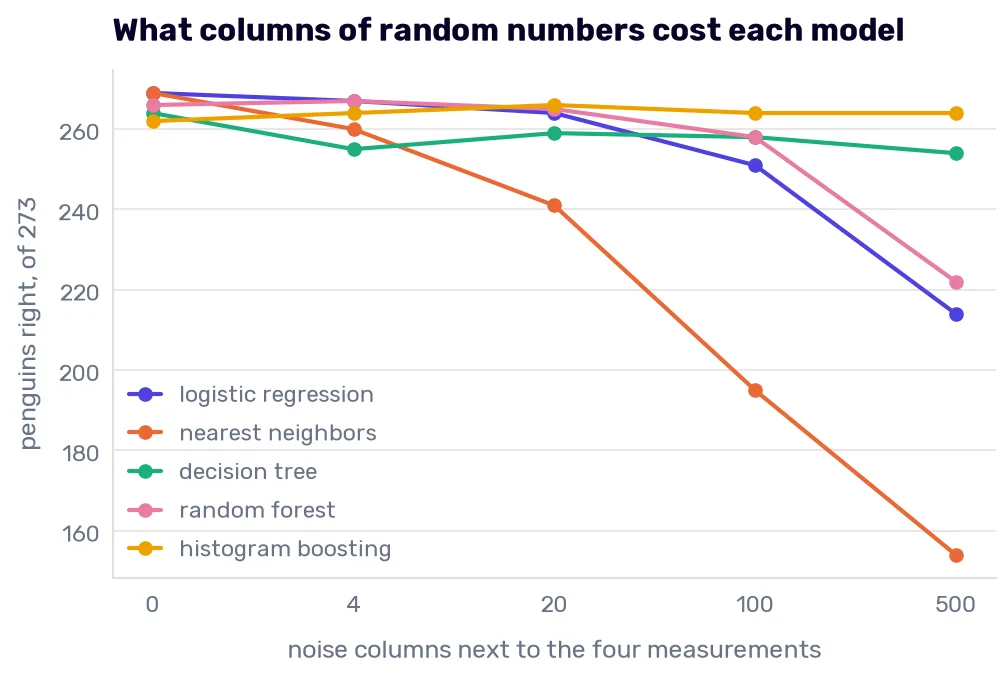
The nearest neighbors suffer first and most. With 4 noise columns, they lose 9 penguins, and with 100 they are at 195, close to the 194 of the island rule. The reason is in the distance formula: every column adds its squared difference to the sum, and after scaling, every column has the same spread. With 4 measurements and 4 noise columns, half of every distance is random. With 500 noise columns, the measurements are less than 1% of it, and the five “nearest” penguins are nearly a random draw.
Logistic regression holds out longer. A noise column can’t lower the loss by much, and the default penalty keeps its coefficient small. But small isn’t 0, and there are many of those coefficients. I checked the model with 100 noise columns: the average noise coefficient is 0.08 in absolute value against 0.93 for the measurements. Every penguin’s score gets a sum of 100 small random numbers added to it. Their signs differ, so most of it cancels, and what’s left still moves a score by about 1 from penguin to penguin, where the measurements move it by 1.6 to 3.2. That’s enough to tip the penguins near a border.
The single tree loses 5 to 10 penguins and then stops caring. It asks about one column at a time and takes the split that separates the species best, which a noise column rarely offers while a real column still has something to give. Its first splits are on the measurements, and they leave groups that are almost pure. To finish, the tree has to cut the last few odd penguins out of each group, and for that job some noise column does as well as any measurement, by accident. With 100 noise columns, the fully grown tree makes four splits on the measurements and nine on noise columns.
The forest holds up to 20 columns, loses 8 penguins at 100, and falls to 222 at 500 because of the max_features='sqrt' from Forests and bagging. Every split sees a random subset of 22 of the 504 columns, and most of the time none of the four measurements is among them. Histogram boosting shows every split every column, and it isn’t immune to the accident: with 100 noise columns, 1,125 of its 2,026 splits are on noise. But its leaves need at least 20 penguins, so a noise split can’t cut out a single odd bird, and each tree only adds a small correction to the scores. Splits on noise pull in random directions and mostly cancel, and the count doesn’t move.
So “let the model sort it out” is a fair plan for boosted trees and a bad one for anything that measures distances. The rest of this chapter is about sorting the columns out ourselves. The three families of methods are called filters, wrappers, and embedded methods.
For the experiments, we put the 10 candidates and the first 20 noise columns into one table:
thirty = candidates.join(noise.iloc[:, :20])
A real project wouldn’t know which columns are noise. We do, so we can count how many of them each method lets through.
Filters: every column on its own
A filter gives every column a score that says how much the column has to do with the target and keeps the columns with the best scores. No model is trained. Scikit-learn’s two standard scores for classification are f_classif and mutual_info_classif:
from sklearn.feature_selection import f_classif, mutual_info_classif

filled = candidates.fillna(candidates.median())
f_score, p_value = f_classif(filled, species)
whole_numbers = [column in ['egg_day', 'sample_number', 'study_year', 'clutch_complete'] for column in candidates.columns]

pd.DataFrame({
    'F': f_score.round(1),
    'p-value': p_value,
    'mutual information': mutual_info_classif(filled, species, discrete_features=whole_numbers, random_state=42).round(3),
    'right, alone': [right(prepared(LogisticRegression()), candidates[[column]]) for column in candidates.columns],
}, index=candidates.columns).sort_values('F', ascending=False)
| F | p-value | mutual information | right, alone | |
|---|---|---|---|---|
| flipper_length_mm | 503.3 | 8.19686e-92 | 0.658 | 224 |
| culmen_length_mm | 334.6 | 8.24227e-74 | 0.598 | 207 |
| culmen_depth_mm | 312.2 | 5.95088e-71 | 0.592 | 209 |
| body_mass_g | 262 | 5.72597e-64 | 0.5 | 195 |
| delta_13_c | 184.5 | 3.05074e-51 | 0.591 | 188 |
| delta_15_n | 164.7 | 1.74064e-47 | 0.436 | 188 |
| egg_day | 45.5 | 9.25332e-18 | 0.633 | 143 |
| sample_number | 20.6 | 4.75003e-09 | 0.316 | 117 |
| clutch_complete | 4.5 | 0.0117219 | 0.015 | 119 |
| study_year | 0.3 | 0.720459 | 0.007 | 121 |
(Neither function accepts a NaN, so the isotopes get their median here. mutual_info_classif treats every column as a continuous measurement unless told otherwise, so whole_numbers marks the four columns that hold counts, dates, and flags. The last column of the table is a logistic regression trained on that one column. The dummy gets 121.)
The F score
The F score compares two kinds of variation in a column. With \(K\) species and \(n\) penguins, where \(n_k\) is the size of species \(k\), \(\bar{x}_k\) its average, and \(\bar{x}\) the average of everybody:
\[F = \frac{\sum_{k} n_k (\bar{x}_k - \bar{x})^2 \,/\, (K - 1)}{\sum_{k} \sum_{i \in k} (x_i - \bar{x}_k)^2 \,/\, (n - K)}\]The top is how far the species’ averages are from the overall average. The bottom is how far the penguins are from the average of their own species. Here it is for the flipper:
flipper = train_df['flipper_length_mm']
by_species = flipper.groupby(species, observed=True)

between = (by_species.size() * (by_species.mean() - flipper.mean()) ** 2).sum() / (3 - 1)
within = ((flipper - by_species.transform('mean')) ** 2).sum() / (len(flipper) - 3)
pd.Series({'between the species': between, 'inside a species': within, 'F': between / within}, name='flipper').round(1)
| flipper | |
|---|---|
| between the species | 20911.9 |
| inside a species | 41.5 |
| F | 503.3 |
The three species average 189.7 mm, 196.6 mm, and 217.0 mm, and inside a species the flippers spread by 6 to 7 mm. The averages are far apart compared with that spread, so F is large. If you have taken a statistics course, you know this number as the one-way analysis of variance (ANOVA). The p-value next to it answers the usual question: if the three species had the same average, how often would chance alone produce an F this large?
Read the formula for what it can’t see. F compares averages, so it rewards a column where one species stands far away from the rest. The flipper wins because the Gentoos are 20 to 27 mm away from the other two, and the formula doesn’t notice that the Adelies and the Chinstraps, 7 mm apart, overlap almost completely.
It can also be large for a column that gets no model anywhere. The sample number has a p-value of 0.000000005. A logistic regression trained on it gets 117 penguins right, 4 fewer than the dummy. The averages do differ: the Adelies were numbered from 1 to 152 and the Chinstraps from 1 to 68, so the average Adelie number is twice the average Chinstrap number. But every species starts at 1, and a penguin with number 30 can be anything. A small p-value says the averages differ. Whether the column separates the classes is another question, and with enough rows the averages of almost any column differ a little.
Mutual information
Mutual information asks a broader question: how much less uncertain is the species once you know the column’s value? Uncertainty is measured the same way as the log loss. Before we look at any column, the best we can do is to say the three shares (44%, 36%, 20%), and that guess has a log loss of 1.05. The mutual information is the part of that 1.05 a column can remove. A value of 0 means the column and the species are independent. Mutual information doesn’t care about averages or straight lines, so in principle it catches any kind of dependence.
The flipper removes 0.66 of the 1.05. The egg day has an F score a tenth of the flipper’s, and its mutual information is nearly as high, because a species’ egg days can form separate clumps (the Gentoos have two, two weeks apart), and an average hides that. Take a little off the 0.633, though. It was computed the way discrete columns are, and you are about to see that this way flatters a column with many different values.
The price is that mutual information has to be estimated, and the estimate is shaky. Scikit-learn does it with nearest neighbors (if penguins with similar flippers tend to have the same species, the two are related), and it adds a little random jitter to the column first, which is why the function takes a random_state.
The sample number shows how shaky. The table gives it 0.316, more than half of the bill’s score. We can work out what it should be. A number above 68 rules out a Chinstrap, a number above 124 leaves only the Adelies, and at 68 or below all three species are about equally likely, whatever the exact number. For a column cut into those three ranges, the mutual information can be counted exactly, with no estimating:
from sklearn.metrics import mutual_info_score

ranges = pd.cut(candidates['sample_number'], [0, 68, 124, 152], labels=['1-68', '69-124', '125-152'])
pd.crosstab(ranges, species)
| sample_number | Adelie | Chinstrap | Gentoo |
|---|---|---|---|
| 1-68 | 56 | 54 | 54 |
| 69-124 | 42 | 0 | 44 |
| 125-152 | 23 | 0 | 0 |
round(float(mutual_info_score(ranges, species)), 3)
0.171
It’s 0.171, and the table said nearly twice that. For a column marked as discrete, the function treats every value as a category of its own, and with 143 different numbers among 273 penguins, no number belongs to more than three birds. A number that only one penguin has predicts that penguin’s species perfectly, on paper. Without the mark, the estimate errs the other way and gives the sample number 0.014. Marking the discrete columns is still the correct call, and a score for a count or an identifier still shouldn’t be compared with the score of a measurement.
(None of this rescues the column. Knowing that a penguin “isn’t a Chinstrap” or “is an Adelie” mostly confirms what the dummy would have guessed anyway, which is why the model on it gets 117.)
The second check is the 20 noise columns:
noise_f, noise_p = f_classif(thirty.iloc[:, 10:], species)
noise_mi = mutual_info_classif(thirty.iloc[:, 10:], species, random_state=42)

pd.Series({
    'smallest p-value': noise_p.min().round(3),
    'p-values below 0.05': (noise_p < 0.05).sum(),
    'largest mutual information': noise_mi.max().round(3),
}, name='the 20 noise columns')
| the 20 noise columns | |
|---|---|
| smallest p-value | 0.007 |
| p-values below 0.05 | 3 |
| largest mutual information | 0.076 |
A column of random numbers gets a mutual information of 0.076. That’s small next to the 0.44 to 0.66 of the measurements and the isotopes, but it isn’t 0, and a weak real column would be hard to tell from it. Of the 20 noise columns, 3 have a p-value below 0.05, and 1 is at 0.007. A p-value below 0.05 is supposed to happen to 1 useless column in 20, so with 500 candidates, 25 would pass on luck. A cutoff on the p-value lets in a fixed share of the noise, however much noise there is.
A third score, chi2, is made for columns of counts and frequencies (how often a word appears in a document). It requires nonnegative values, so it doesn’t fit measurements.
The best k columns
SelectKBest is the filter as a pipeline step. It computes the score for every column, keeps the k best, and drops the rest. Because it’s a step, it’s fitted on the training part of every fold:
from sklearn.feature_selection import SelectKBest

pd.DataFrame({
    k: {
        'logistic regression': right(prepared(SelectKBest(f_classif, k=k), LogisticRegression()), thirty),
        'nearest neighbors': right(prepared(SelectKBest(f_classif, k=k), KNeighborsClassifier(n_neighbors=5)), thirty),
    }
    for k in [1, 2, 3, 4, 6, 8, 10, 15, 30]
}).T.rename_axis('columns kept')
| columns kept | logistic regression | nearest neighbors |
|---|---|---|
| 1 | 224 | 219 |
| 2 | 260 | 261 |
| 3 | 267 | 266 |
| 4 | 269 | 269 |
| 6 | 271 | 272 |
| 8 | 271 | 271 |
| 10 | 271 | 272 |
| 15 | 272 | 266 |
| 30 | 273 | 262 |
With k=6, the filter keeps the four measurements and the two isotopes in every fold, and we are back at 271 and 272. Asking for more brings in the expedition columns and then the noise, which costs the neighbors (266 at 15, 262 at 30).
The bottom row needs a comment. Logistic regression with all 30 columns gets 273 of 273. That’s the egg day and the sample number at work, and I have already said why I don’t believe them.
The top rows show the filter’s blind spot. It scores every column alone, so its best two are the flipper and the bill length (260 and 261), and the best pair in our table of subsets was the two bill columns (264 and 265). Its best three include the flipper, the one column we could drop for free. A filter can’t know that two columns are worth more together than apart, and it can’t know that a column repeats what a better one already said. For the second problem, people add a redundancy check by hand: when two columns correlate above some cutoff, drop one. The flipper and the mass correlate at 0.87 here. It’s the same reasoning as in Choosing what to keep, and it has the same weakness, because which of the two you drop is arbitrary.
Where the selection goes
SelectKBest looked at the species to compute its scores. That makes it a step that learns from the target, and you saw in Where the resampling goes what happens when such a step runs before the folds are cut. Here it is once more, on a table built to show it: the flipper, the body mass, and all 500 noise columns.
weak = train_df[['flipper_length_mm', 'body_mass_g']].join(noise)
picked = SelectKBest(f_classif, k=10).fit(weak, species).get_support()
selector_inside = make_pipeline(StandardScaler(), SelectKBest(f_classif, k=10), KNeighborsClassifier(n_neighbors=5))

pd.Series({
    'the flipper and the mass, no selection': right(species_knn, weak.iloc[:, :2]),
    'best 10 picked on all rows, then cross-validated': right(species_knn, weak.loc[:, picked]),
    'best 10 picked inside every fold': right(selector_inside, weak),
}, name='right, of 273')
| right, of 273 | |
|---|---|
| the flipper and the mass, no selection | 223 |
| best 10 picked on all rows, then cross-validated | 214 |
| best 10 picked inside every fold | 193 |
Picked on all 273 rows, the best 10 columns are the flipper, the mass, and 8 noise columns. Those 8 were chosen because, by accident, their values line up a little with the species, and “all 273 rows” includes the rows of every validation part. So the accident holds on the validation rows too, and the folds report 214.
Inside the folds, the selector sees only the training part. It still picks noise columns, different ones each time (26 different columns across the 5 folds, and only 3 of them in all 5), but now their accidents don’t extend to the validation rows. The count is 193, and that’s what this procedure is worth. The first number overstated it by 21 penguins.
Both numbers are below the 223 we get without the noise, so the 214 would never have looked like a triumph. It didn’t have to. It only had to look better than the alternatives on your list, and an estimate that’s 21 penguins too kind will do that.
I owe you the other side as well. When I swap the flipper and the mass for all four measurements and repeat the experiment, the two counts are 261 and 257 for the neighbors, and 269 and 270 for the logistic regression. With strong columns in the table, the selector finds them every time. The leak shrinks to four penguins for the neighbors and disappears for the logistic regression. The leak grows with the number of candidates and shrinks with the strength of the real columns, and the genomics and text datasets where people select 50 columns from 20,000 with a few hundred rows are at the bad end of both. On data like that, selecting first can produce a good-looking score from columns that hold nothing at all.
Wrappers: the model’s score chooses
A wrapper doesn’t score columns. It trains the model on different subsets and keeps the subset on which the model does best. We did that in Every subset of four columns with all 15 of them. With 30 columns and a billion subsets, the search needs a shortcut, and each wrapper is a different shortcut.
Recursive feature elimination
Recursive feature elimination (RFE) starts with every column. It trains the model, finds the column with the smallest coefficients, drops it, and trains again on what is left. It repeats that until the number of columns you asked for remains:
from sklearn.feature_selection import RFE, RFECV

def kept_in_folds(pipeline, table=thirty):
    kept = []
    for train_rows, _ in folds.split(table, species):
        fitted = clone(pipeline).fit(table.iloc[train_rows], species.iloc[train_rows])
        kept.extend(table.columns[fitted[-2].get_support()])
    return pd.Series(kept).value_counts()

rfe = prepared(RFE(LogisticRegression(), n_features_to_select=6), LogisticRegression())
kept = {
    'F score, best 6': kept_in_folds(prepared(SelectKBest(f_classif, k=6), LogisticRegression())),
    'RFE, 6': kept_in_folds(rfe),
}
right(rfe, thirty)
272
kept_in_folds() fits a pipeline on the training part of every fold and counts how often the selector (the step before the model) kept each column. We collect those counts for Do the methods agree?.
For a model with three rows of coefficients, “the smallest” means the smallest sum of squares over the three species. Comparing coefficients across columns only makes sense when the columns share a scale, so the scaler in front is required. RFE also works with a forest, where it drops the column with the lowest feature_importances_.
Retraining after every drop matters. In Reading the coefficients, correlated columns shared their coefficients, so two columns that carry the same information can both look small. Once one of them is gone, the other inherits its share and survives the next round. Dropping the 24 smallest columns in one go would throw both away.
RFE needs to be told how many columns to keep. RFECV chooses the number with a cross-validation of its own, run inside the training part it’s given:
inner_folds = StratifiedKFold(n_splits=5, shuffle=True, random_state=0)
rfecv = prepared(RFECV(LogisticRegression(), cv=inner_folds, scoring='balanced_accuracy'), LogisticRegression())
kept['RFECV'] = kept_in_folds(rfecv)

sizes = [
    clone(rfecv).fit(thirty.iloc[train_rows], species.iloc[train_rows])[-2].n_features_
    for train_rows, _ in folds.split(thirty, species)
]
pd.Series({'right, of 273': right(rfecv, thirty), 'columns kept in the five folds': ', '.join(map(str, sizes))}, name='RFECV')
| RFECV | |
|---|---|
| right, of 273 | 270 |
| columns kept in the five folds | 9, 8, 9, 5, 8 |
270 right, and the five folds kept 9, 8, 9, 5, and 8 columns. Folds inside folds are the nested cross-validation I mentioned in one parenthesis in Regularization and tuning. The inner folds choose, and the outer folds measure the whole procedure, the choosing included, which is what Rule 29 asked for.
Sequential selection
RFE trusts the coefficients. SequentialFeatureSelector trusts only the score, so it works with any model, the nearest neighbors included. Going forward, it starts with no columns, tries each one alone, and keeps the one with the best cross-validated score. Then it tries each remaining column next to the first, keeps the best pair, and so on. Going backward, it starts with all columns and removes the one whose absence hurts least.
from sklearn.feature_selection import SequentialFeatureSelector

def sequential(direction):
    selector = SequentialFeatureSelector(
        KNeighborsClassifier(n_neighbors=5), n_features_to_select=6, direction=direction,
        cv=inner_folds, scoring='balanced_accuracy',
    )
    return prepared(selector, KNeighborsClassifier(n_neighbors=5))

kept['forward, 6'] = kept_in_folds(sequential('forward'))
kept['backward, 6'] = kept_in_folds(sequential('backward'))

pd.Series({direction: right(sequential(direction), thirty) for direction in ['forward', 'backward']}, name='right, of 273')
| right, of 273 | |
|---|---|
| forward | 271 |
| backward | 270 |
Both get about what the filter got. The difference is the cost. To choose 6 of 30 columns going forward, the selector scores 30 candidates, then 29, down to 25, which is 165 candidates. Each is scored on five inner folds, and all of it happens once per outer fold, so one forward run over the five folds trains 4,125 models. The backward run has to remove 24 columns and trains 11,100. The penguins take seconds. With a table of a million rows and a model that needs a minute to train, the forward run alone is three days.
The search is also greedy. In the forward direction, the first pick is the column that scores best alone on the inner folds (the delta_13_c, in all five of ours), and whatever is picked stays for good. Nothing guarantees that the best single column belongs to the best pair. In our table of subsets, the flipper was the best column alone, and the best pair didn’t contain it. A column that’s only useful together with another can’t get in on its own either. Going backward avoids the second problem, because the columns that work together start out together. It’s just as greedy (a dropped column never comes back), and it costs more.
And there is the winner’s curse, built in this time. At every step, the selector picks the best of up to 30 scores. Each score is an average over five inner folds of about 44 penguins, 218 in all, so one penguin moves it by about half a percentage point. With that many tries and candidates that close together, luck picks some of the winners. You will see which in Do the methods agree?.
Embedded methods: the model chooses while it trains
Some models select columns as a side effect of training, and those are the embedded methods. You have met the first one. In Regularization and tuning, Lasso’s absolute-value penalty pushed coefficients all the way to 0, and the columns with a 0 were out of the model.
Logistic regression has the same penalty. Since scikit-learn 1.8, you ask for it with l1_ratio=1 (the older penalty='l1' is deprecated), and it needs the saga solver, which shuffles the rows as it goes (hence the random_state). C works as before, and a smaller C means a stronger penalty:
sparse_models = {}
for C in [0.01, 0.03, 0.1, 0.3, 1, 10]:
    sparse = prepared(LogisticRegression(l1_ratio=1, C=C, solver='saga', max_iter=10000, random_state=42))
    nonzero = (sparse.fit(thirty, species)[-1].coef_ != 0).any(axis=0)
    sparse_models[C] = {
        'real columns kept': nonzero[:10].sum(),
        'noise columns kept': nonzero[10:].sum(),
        'right': right(sparse, thirty),
    }

pd.DataFrame(sparse_models).T.rename_axis('C')
| C | real columns kept | noise columns kept | right |
|---|---|---|---|
| 0.01 | 3 | 0 | 121 |
| 0.03 | 5 | 0 | 264 |
| 0.1 | 7 | 0 | 268 |
| 0.3 | 7 | 0 | 270 |
| 1 | 7 | 3 | 271 |
| 10 | 9 | 6 | 271 |
The table reads from the strongest penalty to the weakest. At 0.01, 3 columns survive with coefficients so small that the model answers “Adelie” for everybody. From 0.03 on, the model works, and up to 0.3 it uses 5 to 7 real columns and none of the 20 noise columns. At the default of 1, the first 3 noise columns get in.
Look at what the model at 0.1 kept:
sparse = prepared(LogisticRegression(l1_ratio=1, C=0.1, solver='saga', max_iter=10000, random_state=42)).fit(thirty, species)
pd.DataFrame(sparse[-1].coef_, index=sparse[-1].classes_, columns=thirty.columns).loc[:, lambda table: (table != 0).any()].round(2)
| culmen_length_mm | culmen_depth_mm | flipper_length_mm | body_mass_g | delta_15_n | delta_13_c | egg_day | |
|---|---|---|---|---|---|---|---|
| Adelie | -1.95 | 0.22 | 0 | 0 | 0 | 0 | -0.06 |
| Chinstrap | 0 | 0 | 0 | 0 | 0 | 1.32 | 0 |
| Gentoo | 0 | -1.37 | 0.61 | 0.21 | -0.12 | 0 | 0 |
Under this penalty, the model describes each species with as few columns as it can. An Adelie is a short bill. A Gentoo is a shallow bill and a long flipper. And a Chinstrap is one number, the delta_13_c. The column we didn’t have until this chapter is the only one the model wants for the species we kept missing.
The penalized model doesn’t have to be the final model. SelectFromModel turns any model with coefficients or importances into a selection step: it fits the model, keeps the columns that pass a threshold, and hands them to the next step. For an L1-penalized model, the threshold is “not zero”:
from sklearn.feature_selection import SelectFromModel

l1_selector = SelectFromModel(LogisticRegression(l1_ratio=1, C=0.1, solver='saga', max_iter=10000, random_state=42))
l1_then_neighbors = prepared(l1_selector, KNeighborsClassifier(n_neighbors=5))
kept['L1, C=0.1'] = kept_in_folds(l1_then_neighbors)

right(l1_then_neighbors, thirty)
273
The nearest neighbors, the model that 20 noise columns hurt most, get all 273 penguins right when a penalized logistic regression chooses their columns first. The selector kept six or seven columns per fold, and none of them was noise. One caution about the 273: in two of the five folds, the seventh column was the egg day.
A forest can play the same role with its feature_importances_, but look at the importances first:
importance = pd.Series(
    clone(forest).fit(thirty.fillna(thirty.median()), species).feature_importances_, index=thirty.columns,
)

pd.concat([importance.iloc[:10], pd.Series({
    'the 20 noise columns together': importance.iloc[10:].sum(),
    'the largest noise column': importance.iloc[10:].max(),
    'the smallest noise column': importance.iloc[10:].min(),
})]).round(4).rename('impurity importance')
| impurity importance | |
|---|---|
| culmen_length_mm | 0.2086 |
| culmen_depth_mm | 0.1444 |
| flipper_length_mm | 0.1617 |
| body_mass_g | 0.0848 |
| delta_15_n | 0.0785 |
| delta_13_c | 0.1226 |
| egg_day | 0.076 |
| sample_number | 0.0251 |
| study_year | 0.0031 |
| clutch_complete | 0.0004 |
| the 20 noise columns together | 0.095 |
| the largest noise column | 0.0088 |
| the smallest noise column | 0.0031 |
The 20 noise columns collect 9.5% of the importance between them, more than the body mass. Every one of them outranks the clutch column, and the weakest ties with the study year. Those two real columns are useless too, but a column of random numbers has 273 different values and so offers 272 places to cut, while the clutch column offers 1. Deep in a tree, where a few penguins are left, one of 272 cuts will separate them by accident, and the importance records the accident as a contribution.
SelectFromModel with a forest keeps the columns above the average importance, which is 1/30 here. That threshold is high enough to cut every noise column:
forest_selector = SelectFromModel(RandomForestClassifier(n_estimators=500, random_state=42))
forest_then_neighbors = prepared(forest_selector, KNeighborsClassifier(n_neighbors=5))
kept['forest, above the mean'] = kept_in_folds(forest_then_neighbors)

right(forest_then_neighbors, thirty)
273
It keeps seven columns in every fold, the egg day among them, and the neighbors get 273 again.
Noise as a yardstick
The noise columns were meant as a trap, and they turn out to be a measuring tool. Any score a column of random numbers can reach is a score that means nothing. Here is the permutation importance from Which measurements decide? on the table of 30:
def probe_importance(model, table=thirty):
    importances = []
    for train_rows, validation_rows in folds.split(table, species):
        fitted = clone(model).fit(table.iloc[train_rows], species.iloc[train_rows])
        result = permutation_importance(
            fitted, table.iloc[validation_rows], species.iloc[validation_rows],
            scoring='balanced_accuracy', n_repeats=30, random_state=42,
        )
        importances.append(result.importances_mean)
    return pd.Series(np.mean(importances, axis=0), index=table.columns)

probes = pd.DataFrame({
    'nearest neighbors': probe_importance(prepared(KNeighborsClassifier(n_neighbors=5))),
    'logistic regression': probe_importance(prepared(LogisticRegression())),
})
pd.concat([probes.iloc[:10], pd.DataFrame({
    'the largest noise column': probes.iloc[10:].max(),
    'the smallest noise column': probes.iloc[10:].min(),
}).T]).round(3)
| nearest neighbors | logistic regression | |
|---|---|---|
| culmen_length_mm | 0.083 | 0.126 |
| culmen_depth_mm | 0.05 | 0.063 |
| flipper_length_mm | 0.02 | 0.013 |
| body_mass_g | 0.011 | 0.009 |
| delta_15_n | 0.033 | 0.012 |
| delta_13_c | 0.073 | 0.066 |
| egg_day | 0.039 | 0.03 |
| sample_number | 0.025 | 0.036 |
| study_year | -0.016 | 0.006 |
| clutch_complete | 0.001 | 0 |
| the largest noise column | 0.013 | 0.004 |
| the smallest noise column | -0.017 | 0 |
For the nearest neighbors, shuffling a noise column moves the balanced accuracy by anything from −0.017 to +0.013. (A negative importance means the model did better with the column shuffled, which can only be luck.) So for this model, an importance inside that band is indistinguishable from nothing. The body mass (0.011), the clutch, and the study year are inside it. The delta_13_c is the second most important column for both models, right behind the bill length.
You can do this on any dataset: add a few columns of random numbers (or shuffled copies of real columns), run your importance method, and distrust every real column that doesn’t beat them. A method called Boruta packages the idea. It adds a shuffled copy of every column, trains a forest, keeps the columns that beat the best shuffled copy, and repeats until the answer is stable. It lives in a separate library, and the few lines above get you most of the way.
Do the methods agree?
Here is how many of the five folds each method kept each column in:
pd.DataFrame(kept).reindex(thirty.columns).dropna(how='all').fillna(0).astype(int)
| F score, best 6 | RFE, 6 | RFECV | forward, 6 | backward, 6 | L1, C=0.1 | forest, above the mean | |
|---|---|---|---|---|---|---|---|
| culmen_length_mm | 5 | 5 | 5 | 5 | 5 | 5 | 5 |
| culmen_depth_mm | 5 | 5 | 5 | 5 | 5 | 5 | 5 |
| flipper_length_mm | 5 | 5 | 5 | 4 | 0 | 5 | 5 |
| body_mass_g | 5 | 5 | 5 | 4 | 1 | 5 | 5 |
| delta_15_n | 5 | 1 | 4 | 3 | 2 | 5 | 5 |
| delta_13_c | 5 | 5 | 5 | 5 | 4 | 5 | 5 |
| egg_day | 0 | 4 | 4 | 2 | 4 | 2 | 5 |
| sample_number | 0 | 0 | 4 | 1 | 1 | 0 | 0 |
| study_year | 0 | 0 | 2 | 0 | 0 | 0 | 0 |
| noise_0 | 0 | 0 | 0 | 0 | 1 | 0 | 0 |
| noise_8 | 0 | 0 | 0 | 1 | 0 | 0 | 0 |
| noise_12 | 0 | 0 | 0 | 0 | 1 | 0 | 0 |
| noise_13 | 0 | 0 | 0 | 0 | 1 | 0 | 0 |
| noise_16 | 0 | 0 | 0 | 0 | 2 | 0 | 0 |
| noise_17 | 0 | 0 | 0 | 0 | 1 | 0 | 0 |
| noise_18 | 0 | 0 | 0 | 0 | 1 | 0 | 0 |
| noise_19 | 0 | 0 | 0 | 0 | 1 | 0 | 0 |
All seven methods keep the two bill columns in every fold, and six of the seven keep the delta_13_c every time. The scores they led to were between 270 and 273, which are ties, so the counts can’t rank the methods, and the kept columns are what tells them apart.
The backward search with the nearest neighbors is the unstable one. It dropped the flipper in all five folds and the mass in four, kept the egg day in four, and gave eight seats to seven different noise columns, a different set in every fold. That’s the winner’s curse I announced: with 30 columns and the neighbors, removing one noise column changes the score by a penguin or two in either direction, and the search follows those wobbles. The forward search let one noise column in, in one fold.
The other five methods kept no noise at all. The F filter, the L1 selector, and the forest judge the columns from one pass of scores or one fitted model. RFE refits 24 times, but it ranks by coefficients, which a single penguin barely moves. The sequential searches compare hundreds of cross-validated scores and take the largest, and RFECV does a milder version of the same thing when it picks its number of columns. It’s the only method that kept the study year, and its count wobbles between 5 and 9.
When a method keeps different columns in every fold, don’t average that away. It’s the same message as in Regularization and tuning, where Lasso swapped cylinders for horsepower once the 1978 cars joined: the data can’t decide between those columns, so the choice between them is yours, and it should be made on what the columns mean. The egg day is the example. Four of the seven methods keep it in most folds, because on these three seasons it does help. No selection method can know that it’s the expedition’s calendar.
PCA makes new columns
There is another way to end up with fewer columns, and you have seen it on the cars. In Dimensionality reduction with PCA, principal component analysis replaced five correlated columns with new ones, and I said what it does without showing how. I also wrote that PCA is where eigenvectors finally pay rent, and then I never showed you one.
PCA starts from the standardized columns and their covariance matrix, the table of how every pair of columns varies together. For standardized columns, it’s the correlation matrix (times 273/272, because the scaler divides by the number of rows and np.cov() by one fewer, which is why the four variances further down sum to 4.014 and not to 4, and why this table says −0.49 and −0.6 where A correlation that points the wrong way said −0.48 and −0.59):
from sklearn.decomposition import PCA

standardized = StandardScaler().fit_transform(train_df[numeric])
covariance = np.cov(standardized, rowvar=False)
pd.DataFrame(covariance, index=numeric, columns=numeric).round(2)
| culmen_length_mm | culmen_depth_mm | flipper_length_mm | body_mass_g | |
|---|---|---|---|---|
| culmen_length_mm | 1 | -0.24 | 0.68 | 0.6 |
| culmen_depth_mm | -0.24 | 1 | -0.6 | -0.49 |
| flipper_length_mm | 0.68 | -0.6 | 1 | 0.87 |
| body_mass_g | 0.6 | -0.49 | 0.87 | 1 |
Now, think of a direction as a recipe with one weight per column, such as “0.5 of the bill length, −0.4 of the bill depth, 0.6 of the flipper, 0.5 of the mass”. Multiply a penguin’s four standardized values by the weights, add them up, and the penguin gets one number: its position along that direction. Across all 273 penguins, those numbers have a variance. PCA looks for the direction (with weights whose squares sum to 1, so that no recipe wins by being louder) along which that variance is the largest.
That search has an exact answer, and it’s the piece of linear algebra you were promised. A matrix multiplied by a vector usually gives a vector that points somewhere else. For a few special vectors, it gives the same vector, only stretched, and those are the matrix’s eigenvectors. The stretch factor is the eigenvalue. For a covariance matrix, the eigenvector with the largest eigenvalue is the direction of the largest variance, and the eigenvalue is that variance. The eigenvector with the second-largest eigenvalue is the best direction at a right angle to the first, and so on. NumPy computes them directly:
variances, directions = np.linalg.eigh(covariance)
variances, directions = variances[::-1], directions[:, ::-1].T

pd.DataFrame(directions, columns=numeric, index=[f'direction {number}' for number in range(1, 5)]).assign(variance=variances).round(3)
| culmen_length_mm | culmen_depth_mm | flipper_length_mm | body_mass_g | variance | |
|---|---|---|---|---|---|
| direction 1 | -0.458 | 0.403 | -0.575 | -0.545 | 2.785 |
| direction 2 | 0.599 | 0.797 | 0.008 | 0.077 | 0.77 |
| direction 3 | 0.631 | -0.412 | -0.196 | -0.627 | 0.349 |
| direction 4 | 0.181 | -0.182 | -0.794 | 0.551 | 0.11 |
(eigh() returns the smallest eigenvalue first and the eigenvectors as columns, so the second line reverses the order and turns them into rows.)
And here is scikit-learn:
pca = PCA().fit(standardized)

pd.DataFrame(pca.components_, columns=numeric, index=pca.get_feature_names_out()).assign(
    variance=pca.explained_variance_, share=pca.explained_variance_ratio_,
).round(3)
| culmen_length_mm | culmen_depth_mm | flipper_length_mm | body_mass_g | variance | share | |
|---|---|---|---|---|---|---|
| pca0 | 0.458 | -0.403 | 0.575 | 0.545 | 2.785 | 0.694 |
| pca1 | 0.599 | 0.797 | 0.008 | 0.077 | 0.77 | 0.192 |
| pca2 | 0.631 | -0.412 | -0.196 | -0.627 | 0.349 | 0.087 |
| pca3 | -0.181 | 0.182 | 0.794 | -0.551 | 0.11 | 0.027 |
The same numbers. The first and the last direction have every sign flipped, which changes nothing: a direction and its opposite are the same line, and which end gets called positive is a convention. NumPy and scikit-learn follow different ones (scikit-learn makes the largest weight of each component positive). So components_ are the eigenvectors of the covariance matrix, explained_variance_ are the eigenvalues, and the share is each eigenvalue divided by their sum.
transform() then does what the recipe said. Take row 182, our stubborn Chinstrap. Standardized, it’s −0.58, −0.28, −0.99, and −1.26: a short bill, a slightly shallow one, a short flipper, and a light bird. Its first component is
Every penguin gets four such numbers, one per direction, and the four new columns are uncorrelated with each other. Nothing is lost while we keep all four, because it’s the same cloud of points seen from a rotated position. The reduction happens when we keep only the first few.
The first direction weighs the bill length, the flipper, and the mass positively and the bill depth negatively. That’s “a big penguin with a shallow bill,” which is a Gentoo, and it holds 69% of the variance:
components = pd.DataFrame(pca.transform(standardized), index=train_df.index, columns=pca.get_feature_names_out())

fig, ax = plt.subplots()
for name, color in SPECIES_COLORS.items():
    rows = components[species == name]
    ax.scatter(rows['pca0'], rows['pca1'], color=color, label=name, s=22, alpha=0.8)
ax.set_title('The penguins on their first two principal components', loc='left')
ax.set_xlabel('first component (69% of the variance)')
ax.set_ylabel('second component (19%)')
ax.legend()
plt.show()
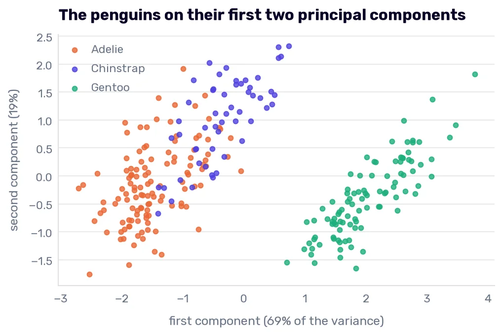
The Gentoos sit alone on the right. The Chinstraps sit above and to the right of the Adelies, and the two clouds overlap. Two components hold 89% of the variance, so they should be nearly as good as four columns:
pd.DataFrame({
    k: {
        'logistic regression': right(make_pipeline(StandardScaler(), PCA(n_components=k), LogisticRegression()), train_df[numeric]),
        'nearest neighbors': right(make_pipeline(StandardScaler(), PCA(n_components=k), KNeighborsClassifier(n_neighbors=5)), train_df[numeric]),
    }
    for k in [1, 2, 3, 4]
}).T.rename_axis('components').assign(**{'share of the variance': pca.explained_variance_ratio_.cumsum().round(3)})
| components | logistic regression | nearest neighbors | share of the variance |
|---|---|---|---|
| 1 | 249 | 245 | 0.694 |
| 2 | 245 | 240 | 0.886 |
| 3 | 269 | 268 | 0.973 |
| 4 | 269 | 269 | 1 |
They aren’t. Two components get 245 and 240, and two of the original columns, the bill length and the bill depth, got 264 and 265. The second component adds nothing to the first and, if anything, costs four or five penguins. The chart shows why. Every species is a cloud stretched along the same rising diagonal, because inside a species a bigger bird scores higher on both components. The Chinstraps are shifted from the Adelies along that diagonal too, so a Chinstrap lands where a large Adelie would. Then the third component, with 9% of the variance, brings 24 penguins.
The cars did the same thing in Dimensionality reduction with PCA. There, a third component with 3% of the variance took the RMSE from 3.67 to 3.50. PCA never sees the target. It ranks directions by how much the penguins spread along them, and the spread that separates an Adelie from a Chinstrap is small next to the spread between small and big penguins. The F score says so too: it’s 1,010 for the first component, 76 for the second, and 86 for the third.
So “keep the components that explain 90% of the variance” is a rule about the inputs, and it can throw away the part you needed. Here, a 90% rule would have kept the third component by a hair, and an 85% rule would have cost 24 penguins. If you use PCA in front of a model, the number of components is one more setting to choose on the folds.
Two more things PCA doesn’t do. It doesn’t forgive unscaled columns: without the scaler, the first component is the body mass, with 99.99% of the variance, and two components give the neighbors 203. And it doesn’t remove noise:
noisy = train_df[numeric].join(noise.iloc[:, :20])

pd.Series({
    'all 24 columns': right(species_knn, noisy),
    **{
        f'{k} components': right(make_pipeline(StandardScaler(), PCA(n_components=k), KNeighborsClassifier(n_neighbors=5)), noisy)
        for k in [2, 4, 8, 16]
    },
}, name='right, of 273')
| right, of 273 | |
|---|---|
| all 24 columns | 241 |
| 2 components | 237 |
| 4 components | 228 |
| 8 components | 223 |
| 16 components | 233 |
With 20 noise columns next to the measurements, every number of components does worse than no PCA. A noise column has a variance of 1 after scaling, as much as a measurement, and it correlates with nothing, so there is no direction that summarizes it. PCA has to keep it, and it takes 19 components to reach 90% of the variance. PCA compresses columns that repeat each other. The decision that a column is useless needs the target, and PCA doesn’t have it.
(There is a relative of PCA that does look at the target. Linear discriminant analysis searches for the directions that separate the classes best, which is the F score’s idea applied to combinations of columns. Its two directions in front of the nearest neighbors get 271 on the four measurements and 269 with the 20 noise columns added.)
When is PCA the right tool, then? When many columns measure nearly the same thing (pixels, sensor readings, survey answers) and when you need a picture. The chart above is the best two-dimensional view of four columns we can get from a rotation, and The Skodas in PCA space was a picture too. As a way of choosing features, PCA has the cost I named on the cars: a coefficient on “0.46 of the bill length minus 0.40 of the bill depth” can’t be checked against anything a biologist knows.
What the model gets
We had 10 candidates, and here is where each of them ends up.
The sample number, the study year, and the clutch stay out. The first is the answer in disguise, and the other two don’t help. The egg day helps by two or three penguins, four selection methods wanted it, and it passed the season test. I leave it out anyway, and the case is thinner than the island’s was. I can’t explain the Gentoos’ two weeks, all three seasons come from one research station, and a bird measured away from its nest has no egg day at all.
The four measurements stay. We could drop the flipper and lose nothing, and I keep it anyway. A tie isn’t a reason to change a model that’s already tested, and four columns that come off a ruler and a scale cost nothing to collect.
The isotopes are the hard case. They describe the penguin, six of the seven selection methods keep the delta_13_c in every fold (the delta_15_n does worse, RFE drops it in four folds of five), and they get rows 182 and 172 right, which no model could do with the four measurements. They also drift between seasons, enough to cancel what they give the nearest neighbors, and they need a blood sample and a mass spectrometer. In What the island and the sex are worth, we worked out that a new penguin arrives without a DNA test, and a bird without a DNA test doesn’t have an isotope analysis either. A column the model won’t get at prediction time can’t be a feature, whatever it does on the folds.
So the species model keeps its four measurements, and what this chapter adds is a price tag. For the logistic regression, a blood sample is worth 2 or 3 penguins in 273, even in a season the model hasn’t seen. For the nearest neighbors, it’s worth 3 penguins on familiar seasons and nothing on an unfamiliar one. Whether that’s worth a needle, a lab, and a wait is a question for the person who has to catch the penguin. It’s the first step of the machine learning process coming back at the end: a feature has a cost, and somebody other than the model has to decide whether to pay it.
No look at the test set
The model we would ship didn’t change, so there is nothing to spend a look on (Rule 14). It also got 69 of 69 the last time, and no look could show an improvement on that.
Along the way, I made a lot of choices by hand. Six columns for the filter and the wrappers. A C of 0.1 for the selector. Five neighbors, because it’s the default. Each of them is a setting I picked from a short table or left at its default, and each could be chosen by a search inside the folds, the way RFECV chose its number of columns. Those searches are the subject of the next chapter.