
Our best model was wrong about 3 of the 54 Chinstraps and about 1 of the other 219 penguins, and the Chinstraps are the species we have the fewest of. Making every species count the same during training won back one penguin, which I called a tie. Then I promised to treat the penguins as an imbalanced dataset anyway.
Why pretend? Because a rare answer is the normal case at work. Fraud is rare among payments, and a broken part is rare on a production line. A dataset like that would need its own exploration chapter, and we know these birds by now. So the penguins stand in, and I will say where a truly rare class would behave differently.
The tools come from a separate library, imbalanced-learn.
How imbalanced are the penguins?
counts = species.value_counts()
pd.DataFrame({'penguins': counts, 'share': (counts / len(species)).round(3)})
| species | penguins | share |
|---|---|---|
| Adelie | 121 | 0.443 |
| Gentoo | 98 | 0.359 |
| Chinstrap | 54 | 0.198 |
In my workshops, I show a rule of thumb: the classes are imbalanced when one of them has 20% of the rows or fewer. The Chinstraps have 19.8%, so by the rule we are in.
The rule deserves two warnings. It’s a convention, and you will meet other cutoffs. It was also made for two classes. With two classes, an even split is 50%, and a class at 20% is outnumbered 4 to 1. With three classes, an even split is 33%, and our Chinstraps are outnumbered 2.2 to 1 by the Adelies and 1.8 to 1 by the Gentoos, which is mild.
The rule fits better when we go back to the question from One question at a time: is this penguin a Chinstrap? That question has two answers. The answer is yes for 54 penguins and no for 219, and the yes is 19.8% of the table. For most of this chapter, that question is our imbalanced problem. The three-species model comes along as a second check on every method.
Keep the scale in mind, though. In fraud detection, the positive class can be 0.1% of the rows. Near the end of the chapter, we will take most of the Chinstraps away from the model to see what that does.
What a model does to a rare class
First, a model for the yes-or-no question:
is_chinstrap = (species == 'Chinstrap').to_numpy()

def chinstrap_share(model, columns=numeric):
    return cross_val_predict(model, train_df[columns], is_chinstrap, cv=folds, method='predict_proba')[:, 1]

def report(share, threshold=0.5):
    said = share > threshold
    return pd.Series({
        'found': (said & is_chinstrap).sum(),
        'missed': (~said & is_chinstrap).sum(),
        'false alarms': (said & ~is_chinstrap).sum(),
    }, name='penguins')

shares = {'nothing done': chinstrap_share(logistic)}
report(shares['nothing done'])
| penguins | |
|---|---|
| found | 47 |
| missed | 7 |
| false alarms | 2 |
logistic is the pipeline from Logistic regression, a scaler and the model with its defaults. chinstrap_share() returns every penguin’s cross-validated probability of being a Chinstrap, and report() counts the answers at a threshold. The folds are now stratified by the answer, so every validation part has 10 or 11 Chinstraps.
The model misses 7 of the 54 Chinstraps and raises 2 false alarms among the 219 other penguins. That’s a recall of 87% and a precision of 96% (47 of 49). The three-species model found 51 Chinstraps, but it’s a different model answering a different question, so the two counts don’t have to agree.
Why does the rare class lose? Think about the bill sizes where the two groups overlap, and suppose that in some corner of that overlap one penguin in three is a Chinstrap. A model that has learned this honestly says 0.33 there, and at a threshold of 0.5 the answer is “no” for every penguin in the corner. It’s wrong about a third of them, and it’s still the answer with the fewest mistakes. Wherever the classes mix, the class with more members takes the corner, and a rare class has fewer members in most corners.
So nothing is broken. The model minimizes its loss, the loss counts every penguin once, and when the probabilities are honest, a cut at 0.5 gives the fewest mistakes the model can expect. The trouble starts when a missed Chinstrap costs us more than a false alarm. With rare classes, that’s the usual situation, because finding them is why the model was built.
There are four things you can do about it:
- Oversampling: add rows of the rare class to the training data, either copies of the existing rows or new synthetic ones.
- Undersampling: drop rows of the common class.
- Class weights: leave the rows alone and tell the model that a mistake on the rare class costs more (when the model supports it).
- Pretending the problem doesn’t exist. It’s the most popular method by far, and sometimes it’s even the correct one.
We will try all four.
Copies of the Chinstraps
The simplest way to get more Chinstraps is to use the ones we have more than once. RandomOverSampler draws rows of every smaller class at random, with replacement, until each class is as large as the largest one:
from imblearn.over_sampling import RandomOverSampler

oversampler = RandomOverSampler(random_state=42)
oversampled, oversampled_species = oversampler.fit_resample(train_df[numeric], species)
oversampled_species.value_counts()
| species | count |
|---|---|
| Adelie | 121 |
| Chinstrap | 121 |
| Gentoo | 121 |
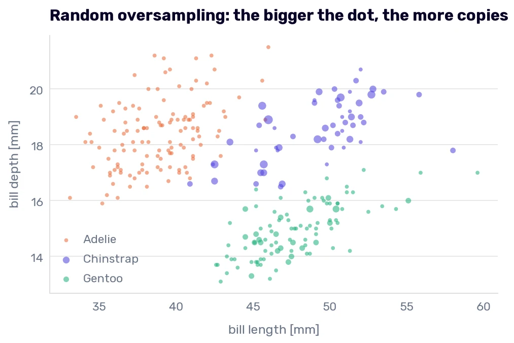
The table grew from 273 rows to 363. There are 67 new Chinstrap rows and 23 new Gentoo rows, and every one of them is a copy of a penguin that was already there. The sampler remembers which rows it drew, so we can count how many times each penguin appears now and draw the count as the size of its dot:
copies = np.bincount(oversampler.sample_indices_, minlength=len(train_df))

fig, ax = plt.subplots()
for name, color in SPECIES_COLORS.items():
    rows = (species == name).to_numpy()
    ax.scatter(train_df.loc[rows, bill[0]], train_df.loc[rows, bill[1]], s=14 * copies[rows], color=color, alpha=0.55, linewidths=0, label=name)
ax.set_title('Random oversampling: the bigger the dot, the more copies', loc='left')
ax.set_xlabel('bill length [mm]')
ax.set_ylabel('bill depth [mm]')
ax.legend()
plt.show()
pd.Series(copies[is_chinstrap], name='times in the table').value_counts().sort_index().rename('Chinstraps')
| times in the table | Chinstraps |
|---|---|
| 1 | 14 |
| 2 | 21 |
| 3 | 12 |
| 4 | 6 |
| 5 | 1 |
The draw is uneven. Of the 54 Chinstraps, 14 appear once, 21 twice, 12 three times, 6 four times, and 1 five times.
No information was added. The model sees the same 54 birds, and some of them now count for more. What that does depends on the model. A logistic regression adds up a loss over the rows, so a penguin that appears three times pulls on the coefficients three times as hard. For the nearest neighbors, a penguin that appears three times takes three of the five seats in every vote it attends.
Before we score anything, we have to decide where in the process the copies get made.
Where the resampling goes
Here is the mistake that’s easy to make. We have a balanced table, so let’s cross-validate a model on it. I take a single nearest neighbor, because it shows the problem best:
one_neighbor = make_pipeline(StandardScaler(), KNeighborsClassifier(n_neighbors=1))
leaked = cross_val_predict(one_neighbor, oversampled, oversampled_species, cv=folds)
confusion_matrix(oversampled_species, leaked)
array([[119,   2,   0],
       [  0, 121,   0],
       [  0,   0, 121]])
Every one of the 121 Chinstraps is found, and 361 of the 363 rows are right. In Nearest neighbors, three species, the same model got 267 of 273.
Nothing improved. The folds were cut after the copies were made, so a penguin and its copy often land on different sides of the cut. Of the 363 rows, 131 were validated by a model that had the very same row in its training part. One nearest neighbor finds that twin at a distance of 0 and reads the answer off it.
The count is wrong too. Of the 363 “penguins” we scored, 90 don’t exist, and the Chinstraps are a third of that table when they are a fifth of the penguins we measured. Even without the twins, the score would describe a population nobody will ever meet.
So the resampling follows the same law as the scaler and the imputer. It happens after the split and touches the training rows only, which gives the test set three things:
- There is no leak. A copy or a synthetic row made from a test penguin never reaches the training data.
- The test set keeps the real class shares, so the score describes the birds the model will meet.
- The experiments stay comparable. We can swap one resampling method for another, and the rows we score on don’t change.
The same holds for every fold of the cross-validation, so the sampler belongs in the pipeline. Scikit-learn’s pipeline can’t hold one. Its steps may change the columns, but they can’t add or remove rows, and a sampler has to run during fit() and stand aside during predict(). Imbalanced-learn ships its own pipeline that does both:
from imblearn.pipeline import make_pipeline as make_sampling_pipeline

def resampled(sampler, model):
    return make_sampling_pipeline(StandardScaler(), sampler, model)

inside = resampled(RandomOverSampler(random_state=42), KNeighborsClassifier(n_neighbors=1))
confusion_matrix(species, cross_val_predict(inside, train_df[numeric], species, cv=folds))
array([[119,   2,   0],
       [  4,  50,   0],
       [  0,   0,  98]])
Now the copies are made inside each fold, from the training part alone, and the validation part holds real penguins in their real proportions. The result is 267 of 273, with 50 of the 54 Chinstraps found. That’s what the single neighbor got without any resampling, and it couldn’t be otherwise: a copy sits in the same spot as its original, so the nearest neighbor of a new penguin is the same bird either way.
With that settled, the copies can be scored on the Chinstrap question:
shares['random oversampling'] = chinstrap_share(resampled(RandomOverSampler(random_state=42), LogisticRegression()))
report(shares['random oversampling'])
| penguins | |
|---|---|
| found | 52 |
| missed | 2 |
| false alarms | 8 |
Five more Chinstraps are found, and there are six more false alarms.
Class weights
If a penguin that appears three times pulls three times as hard, we can skip the copying and hand the model the multiplier. That is what class_weight does, the setting I used without much explanation at the end of The first classifiers and their mistakes. With 'balanced', class \(k\) gets the weight
where \(n\) is the number of rows, \(K\) the number of classes, and \(n_k\) the size of the class:
from sklearn.utils.class_weight import compute_class_weight

labels = np.unique(species)
pd.Series(compute_class_weight('balanced', classes=labels, y=species), index=labels, name='weight').round(2)
| weight | |
|---|---|
| Adelie | 0.75 |
| Chinstrap | 1.69 |
| Gentoo | 0.93 |
A Chinstrap gets 273 / (3 × 54) = 1.69. Each weight times the size of its class gives 91, a third of the 273 rows, for all three species.
Inside the model, the weight multiplies the penguin’s term in the log loss. A mistake on a Chinstrap now costs 1.69 times what it did, and a mistake on an Adelie 0.75 times. The ratio of the two is 2.24, the same as 121 to 54, so the weights do what random oversampling does on average, without the dice. For the Chinstrap question, the weights are 2.53 for a yes and 0.62 for a no:
weighted = make_pipeline(StandardScaler(), LogisticRegression(class_weight='balanced'))
shares['class weights'] = chinstrap_share(weighted)
report(shares['class weights'])
| penguins | |
|---|---|
| found | 53 |
| missed | 1 |
| false alarms | 8 |
It finds 53 of the 54 with the same 8 false alarms, which is a tie with the copies.
Not every model takes the setting. LogisticRegression, the trees, the forest, and HistGradientBoostingClassifier have class_weight. KNeighborsClassifier doesn’t, because it has no loss to weight.
Synthetic penguins
Copies add nothing new, so the next idea is to invent Chinstraps that look plausible. The best-known method is SMOTE, the Synthetic Minority Over-sampling Technique. For every new penguin, it does this:
- Take a real Chinstrap.
- Find its five nearest neighbors among the other Chinstraps.
- Pick one of the five at random.
- Put the new penguin at a random point on the straight line between the two.
Here, \(\lambda\) is a random number between 0 and 1, and the same \(\lambda\) is used for all four measurements, so the new penguin stays on the line.
SMOTE looks for neighbors, so it measures distances, and we saw in Nearest neighbors, three species what a body mass in grams does to the distance between two penguins. The sampler goes after the scaler:
from imblearn.over_sampling import SMOTE

scaler = StandardScaler().fit(train_df[numeric])
with_synthetic, with_synthetic_species = SMOTE(random_state=42).fit_resample(scaler.transform(train_df[numeric]), species)

synthetic = pd.DataFrame(scaler.inverse_transform(with_synthetic[len(train_df):]), columns=numeric)
synthetic['species'] = with_synthetic_species[len(train_df):].to_numpy()
synthetic['species'].value_counts()
| species | count |
|---|---|
| Chinstrap | 67 |
| Gentoo | 23 |
The new rows come after the 273 real ones, so everything after the first 273 rows is synthetic. SMOTE made 67 Chinstraps and 23 Gentoos, enough to bring both species to 121. Here are the first three, converted back to millimeters and grams:
synthetic.head(3).round(2)
| culmen_length_mm | culmen_depth_mm | flipper_length_mm | body_mass_g | species | |
|---|---|---|---|---|---|
| 0 | 49.17 | 18.2 | 195 | 4391.4 | Chinstrap |
| 1 | 52.46 | 20.3 | 207.12 | 4655.85 | Chinstrap |
| 2 | 50.87 | 18.4 | 197.39 | 3759.87 | Chinstrap |
Nobody measured these birds. A flipper of 207.12 mm and a body mass of 4655.85 g belong to a point between two real Chinstraps. Nature-identical synthetic penguins, Pengdroids if you will.
fig, axes = plt.subplots(1, 3, figsize=(7.6, 3.6), sharex=True, sharey=True)
for ax, (name, color) in zip(axes, SPECIES_COLORS.items()):
    real = train_df[species == name]
    made = synthetic[synthetic['species'] == name]
    ax.scatter(train_df[bill[0]], train_df[bill[1]], color='#dddddd', s=8)
    ax.scatter(real[bill[0]], real[bill[1]], color=color, s=12, label='real')
    ax.scatter(made[bill[0]], made[bill[1]], facecolors='none', edgecolors='#222222', s=16, linewidths=0.8, label='synthetic')
    ax.set_title(name, loc='left')
    ax.set_xlabel('bill length [mm]')
axes[0].set_ylabel('bill depth [mm]')
fig.legend(*axes[1].get_legend_handles_labels(), loc='upper center', bbox_to_anchor=(0.5, -0.1), ncol=2)
plt.show()
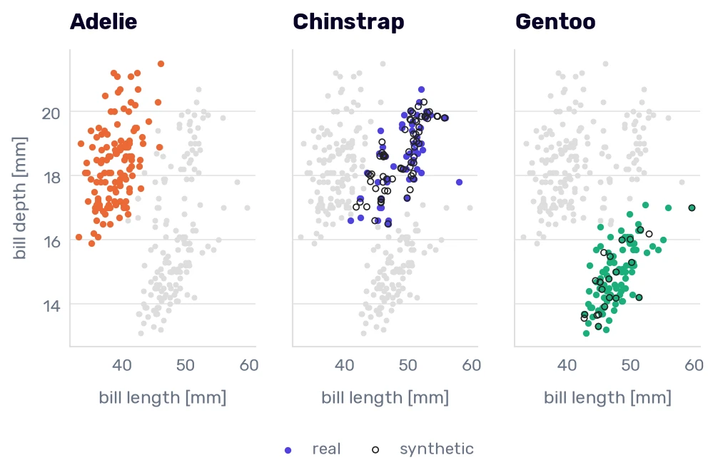
The Adelies are the largest class, so they get no rings. The synthetic Chinstraps fill the inside of the Chinstrap cloud. The neighbors were chosen with all four measurements, so a ring sometimes sits between two Chinstraps that don’t look like neighbors on this chart.
Look at where the rings are missing. No synthetic penguin lies outside the area its species already covers, because a point between two Chinstraps can’t. SMOTE has never seen a Chinstrap that isn’t in the table, and it can’t guess where one would be. In this run, the nearest real penguin of every synthetic one belongs to its own species. That isn’t guaranteed. When a class has an outlier deep in another class’s territory, SMOTE draws lines to it and puts synthetic rows along the way.
SMOTE needs numbers to draw a line. For a table with categorical columns, there is SMOTENC, which interpolates the numbers and gives the new row the most frequent category among the neighbors. Two more variants spend the synthetic rows where the classes meet. BorderlineSMOTE builds only from the rare rows that have many, but not only, neighbors of other classes, and ADASYN makes more rows around the rare rows that are surrounded by other classes.
The score on the Chinstrap question:
shares['SMOTE'] = chinstrap_share(resampled(SMOTE(random_state=42), LogisticRegression()))
report(shares['SMOTE'])
| penguins | |
|---|---|
| found | 51 |
| missed | 3 |
| false alarms | 6 |
The model trained with the Pengdroids finds 51 Chinstraps and raises 6 false alarms.
Throwing penguins away
We can also balance the classes from the other end. RandomUnderSampler draws 54 penguins from each larger class, without replacement, and drops the rest:
from imblearn.under_sampling import RandomUnderSampler

undersampler = RandomUnderSampler(random_state=42)
kept, kept_species = undersampler.fit_resample(train_df[numeric], species)
kept_species.value_counts()
| species | count |
|---|---|
| Adelie | 54 |
| Chinstrap | 54 |
| Gentoo | 54 |
was_kept = np.isin(np.arange(len(train_df)), undersampler.sample_indices_)

fig, ax = plt.subplots()
ax.scatter(train_df.loc[~was_kept, bill[0]], train_df.loc[~was_kept, bill[1]], color='#cccccc', s=22, label='thrown away')
for name, color in SPECIES_COLORS.items():
    rows = was_kept & (species == name).to_numpy()
    ax.scatter(train_df.loc[rows, bill[0]], train_df.loc[rows, bill[1]], color=color, s=22, label=name)
ax.set_title('Random undersampling: 54 penguins of each species stay', loc='left')
ax.set_xlabel('bill length [mm]')
ax.set_ylabel('bill depth [mm]')
ax.legend()
plt.show()
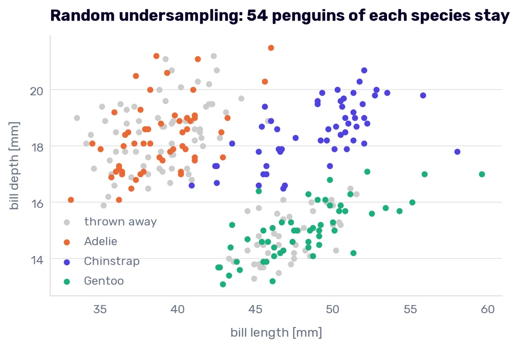
We are left with 162 penguins. The 111 gray dots are real, measured birds (67 Adelies and 44 Gentoos) that the model never sees. On a table of 273 rows, that’s a high price, and there is a second one: the result depends on which penguins the draw keeps.
draws = []
for seed in range(20):
    sampler = RandomUnderSampler(random_state=seed)
    draw = report(chinstrap_share(resampled(sampler, LogisticRegression())))
    draw['three species, right'] = fold_scores(resampled(sampler, LogisticRegression()))['right']
    draws.append(draw)

pd.DataFrame(draws).agg(['min', 'max'])
| found | missed | false alarms | three species, right | |
|---|---|---|---|---|
| min | 50 | 1 | 7 | 268 |
| max | 53 | 4 | 12 | 270 |
Over 20 seeds, the same model on the same data finds between 50 and 53 Chinstraps and raises between 7 and 12 false alarms.
Undersampling makes sense when the common class is huge. With 10 million legitimate payments and 10,000 frauds, dropping nine tenths of the legitimate ones loses little and makes the training much faster. Google’s crash course recommends it for such cases, together with a weight on the kept rows that makes up for the dropped ones.
Cleaning the border
Other undersamplers choose what to remove. Two of them look for penguins that sit too close to another species.
A Tomek link is a pair of penguins of different species that are each other’s nearest neighbor. TomekLinks finds such pairs and removes every member that isn’t in the smallest class (so a pair without a Chinstrap loses both birds). Edited nearest neighbors (EditedNearestNeighbours, in the British spelling) goes further. It removes every penguin outside the smallest class that has a penguin of another species among its three nearest neighbors.
Imbalanced-learn also chains the two ideas. SMOTETomek and SMOTEENN run SMOTE first and one of the cleaners after it. Inside these two, the cleaner is set to remove rows of every class, the smallest one included. The reason given in its documentation is that SMOTE can put synthetic rows between an outlier and the rest of its class, and the cleaning removes the noise this leaves behind.
from imblearn.combine import SMOTEENN, SMOTETomek
from imblearn.under_sampling import EditedNearestNeighbours, TomekLinks

samplers = {
    'random oversampling': RandomOverSampler(random_state=42),
    'SMOTE': SMOTE(random_state=42),
    'random undersampling': RandomUnderSampler(random_state=42),
    'Tomek links': TomekLinks(),
    'edited nearest neighbors': EditedNearestNeighbours(),
    'SMOTE, then Tomek links': SMOTETomek(random_state=42),
    'SMOTE, then edited nearest neighbors': SMOTEENN(random_state=42),
}

scaled = scaler.transform(train_df[numeric])
pd.DataFrame({
    name: sampler.fit_resample(scaled, species)[1].value_counts() for name, sampler in samplers.items()
}).T.assign(rows=lambda table: table.sum(axis=1))
| Adelie | Chinstrap | Gentoo | rows | |
|---|---|---|---|---|
| random oversampling | 121 | 121 | 121 | 363 |
| SMOTE | 121 | 121 | 121 | 363 |
| random undersampling | 54 | 54 | 54 | 162 |
| Tomek links | 119 | 54 | 98 | 271 |
| edited nearest neighbors | 116 | 54 | 98 | 268 |
| SMOTE, then Tomek links | 121 | 121 | 121 | 363 |
| SMOTE, then edited nearest neighbors | 116 | 116 | 121 | 353 |
The cleaners barely touch our table. TomekLinks removes two Adelies:
removed = ~np.isin(np.arange(len(train_df)), samplers['Tomek links'].sample_indices_)
train_df.loc[removed, numeric + ['sex', 'species']]
| culmen_length_mm | culmen_depth_mm | flipper_length_mm | body_mass_g | sex | species | |
|---|---|---|---|---|---|---|
| 73 | 45.8 | 18.9 | 197 | 4150 | MALE | Adelie |
| 131 | 43.1 | 19.2 | 197 | 3500 | MALE | Adelie |
We have met row 73. In The penguins they get wrong, he was one of the Adelie males with a large bill that the models kept calling Chinstraps. His nearest neighbor is a Chinstrap, row 160, another regular of that list. The method found by distance what we found by reading the mistakes.
Its fix is to delete the Adelie, and that deserves a second thought. On paper, rows 73 and 160 are nearly the same bird. Their bills are 45.8 mm and 46.0 mm long, both are 18.9 mm deep, both penguins weigh 4150 g, and the flippers are 197 mm and 195 mm. In Duplicates, I said what to do with a row that has identical features and a different target: don’t delete it, because it’s noise you can’t remove, and it tells you how accurate any model can get. These two aren’t identical, but they are close enough for the same advice. Row 73 is a real bird with the right label, and the next Adelie male with a 45.8-millimeter bill will look just like him. Deleting him makes the border tidier in the training data and leaves the border in the colony where it was.
After SMOTE, the Tomek cleaner finds nothing to remove, and the second cleaner removes five Adelies and five Chinstraps.
Everything side by side
comparison = {}
for name, sampler in {'nothing done': 'passthrough', **samplers}.items():
    shares[name] = chinstrap_share(resampled(sampler, LogisticRegression()))
    comparison[name] = {
        'Chinstraps found': report(shares[name])['found'],
        'false alarms': report(shares[name])['false alarms'],
        'three species, logistic regression': fold_scores(resampled(sampler, LogisticRegression()))['right'],
        'three species, five neighbors': fold_scores(resampled(sampler, KNeighborsClassifier(n_neighbors=5)))['right'],
    }

comparison['class weights'] = {
    'Chinstraps found': report(shares['class weights'])['found'],
    'false alarms': report(shares['class weights'])['false alarms'],
    'three species, logistic regression': fold_scores(weighted)['right'],
    'three species, five neighbors': '',
}
pd.DataFrame(comparison).T
| Chinstraps found | false alarms | three species, logistic regression | three species, five neighbors | |
|---|---|---|---|---|
| nothing done | 47 | 2 | 269 | 269 |
| random oversampling | 52 | 8 | 269 | 266 |
| SMOTE | 51 | 6 | 270 | 265 |
| random undersampling | 52 | 11 | 270 | 264 |
| Tomek links | 47 | 2 | 269 | 269 |
| edited nearest neighbors | 47 | 2 | 269 | 269 |
| SMOTE, then Tomek links | 51 | 6 | 270 | 265 |
| SMOTE, then edited nearest neighbors | 51 | 7 | 269 | 266 |
| class weights | 53 | 8 | 270 |
The first two columns are the Chinstrap question (of 54 Chinstraps and 219 others), and the last two count the right answers of the three-species models out of 273.
Start on the right. With three species, the logistic regression gets 269 or 270 whatever we do, and one penguin is a tie. The five neighbors get worse with every method that balances the classes. With random oversampling, they find one more Chinstrap and lose four Adelies, because the copies vote together, and near the border a few Chinstraps with three seats each outvote the Adelies around them. For the three-species model, pretending the problem doesn’t exist was the correct method. Its mistakes come from penguins whose measurements overlap, as we saw in The penguins they get wrong, and the class sizes have little to do with them.
On the Chinstrap question, every method that balances the classes finds four to six more Chinstraps and pays with four to nine more false alarms, while the two cleaners change nothing.
More Chinstraps found for more false alarms is a trade we have seen before.
It was the threshold
Every method so far retrained the model, on changed data or with changed weights. Here is the untouched model again, with nothing changed but the threshold from Scores and thresholds:
pd.DataFrame({
    threshold: report(shares['nothing done'], threshold) for threshold in [0.5, 0.4, 0.3, 0.25, 0.2]
}).T.rename_axis('threshold')
| threshold | found | missed | false alarms |
|---|---|---|---|
| 0.5 | 47 | 7 | 2 |
| 0.4 | 47 | 7 | 4 |
| 0.3 | 51 | 3 | 5 |
| 0.25 | 53 | 1 | 8 |
| 0.2 | 54 | 0 | 13 |
At 0.25, the untouched model finds 53 Chinstraps with 8 false alarms, which is the result of the class weights to the penguin. At 0.3, it finds 51 with 5, a tie with SMOTE’s 51 with 6.
There is arithmetic behind the match. Balancing takes the Chinstraps from 54 against 219 to one against one, so their odds in the training data are multiplied by 219 / 54 = 4.06, and a logistic regression answers by multiplying the odds it reports by about the same number. Even odds in the balanced world are odds of 1 to 4 in the real one, a probability of 0.2. A balanced model at a threshold of 0.5 behaves roughly like the original model at 0.2. The match isn’t exact (here it lands between 0.2 and 0.3), because the coefficients move a little as well.
If these methods only move the threshold, they shouldn’t change the order in which the model ranks the penguins. The number that measures the order belongs to the precision-recall curve I promised in ROC and AUC. The curve plots the precision against the recall for every threshold, and the average precision sums it up the way the AUC sums up the ROC curve: it’s the mean of the precision over the thresholds, each weighted by the recall it adds. A model that knows nothing gets the share of the positive class, 0.198 here, and a perfect model gets 1.
from sklearn.metrics import average_precision_score

pd.DataFrame({
    name: {
        'average precision': average_precision_score(is_chinstrap, share),
        'mean share': share.mean(),
        'log loss': log_loss(is_chinstrap, share),
    }
    for name, share in shares.items()
}).T.round(3)
| average precision | mean share | log loss | |
|---|---|---|---|
| nothing done | 0.986 | 0.198 | 0.099 |
| random oversampling | 0.988 | 0.248 | 0.105 |
| class weights | 0.986 | 0.253 | 0.117 |
| SMOTE | 0.988 | 0.241 | 0.101 |
| random undersampling | 0.98 | 0.282 | 0.165 |
| Tomek links | 0.985 | 0.2 | 0.099 |
| edited nearest neighbors | 0.987 | 0.203 | 0.099 |
| SMOTE, then Tomek links | 0.988 | 0.241 | 0.101 |
| SMOTE, then edited nearest neighbors | 0.986 | 0.242 | 0.102 |
The average precision is between 0.98 and 0.99 in every row. The models rank the penguins equally well, and each method picked a different place to cut the ranking.
The other two columns show what the move costs. The untouched model’s scores average 0.198, the real share of Chinstraps, which is the first thing to ask of scores that claim to be probabilities (see Is the score a probability?). A logistic regression passes this check almost by construction, because its intercept is fitted so that the scores average to the class share, so passing it proves little. Failing it is enough to distrust the numbers. After balancing, the average is 0.24 to 0.28. Those models were trained in a world with too many Chinstraps and report it faithfully, and the log loss is worse in every balanced row. If anything downstream uses the number itself, like the limit of 0.8 in A second opinion or an expected cost, a resampled model hands it inflated numbers.
from sklearn.metrics import PrecisionRecallDisplay

fig, ax = plt.subplots(figsize=(7.6, 4.8))
PrecisionRecallDisplay.from_predictions(is_chinstrap, shares['nothing done'], name='nothing done, every threshold', curve_kwargs={'color': '#999999'}, ax=ax)
for name, color in zip(['nothing done', 'SMOTE', 'class weights', 'random undersampling'], ['#222222', '#4d41e0', '#eb6834', '#1baf7a']):
    at_half = report(shares[name])
    ax.scatter(
        at_half['found'] / is_chinstrap.sum(), at_half['found'] / (at_half['found'] + at_half['false alarms']),
        color=color, s=50, zorder=3, label=f'{name}, at 0.5',
    )
ax.set_xlim(0.8, 1.005)
ax.set_ylim(0.7, 1.005)
ax.set_xlabel('recall')
ax.set_ylabel('precision')
ax.set_title('Is it a Chinstrap? Four models and one curve', loc='left')
ax.legend(loc='lower left', fontsize=10)
plt.show()
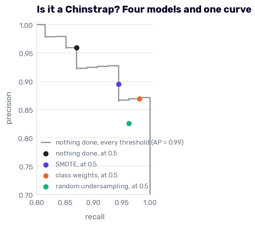
The gray line is the untouched model at every threshold, and the chart shows only the corner where everything happens. The four dots are four models at 0.5. SMOTE and the class weights sit on the line. Undersampling sits a little below it, as you’d expect from a model trained on fewer penguins.
So a model with usable scores doesn’t need any of the samplers.
The rule needs enough positives in the validation data to choose on, and When the class is really rare shows what to do without them.
That, by the way, is what we did in the news-article classification model I told you about in the evaluation step. Every model had a different classification threshold to make up for the fact that relevant news is rather rare.
TunedThresholdClassifierCV chooses the threshold inside the training data. Class weights land in nearly the same place when you’d rather not carry a threshold around. Resampling is what’s left for a model that offers neither.
What resampling can’t do
Let’s take the bill away. Flipper length and body mass can tell a Gentoo from the rest, and they can’t tell an Adelie from a Chinstrap:
weak = ['flipper_length_mm', 'body_mass_g']

weak_shares = {
    'nothing done': chinstrap_share(logistic, weak),
    'class weights': chinstrap_share(weighted, weak),
    'random oversampling': chinstrap_share(resampled(RandomOverSampler(random_state=42), LogisticRegression()), weak),
    'SMOTE': chinstrap_share(resampled(SMOTE(random_state=42), LogisticRegression()), weak),
    'random undersampling': chinstrap_share(resampled(RandomUnderSampler(random_state=42), LogisticRegression()), weak),
}

pd.DataFrame({
    name: {**report(share), 'average precision': round(average_precision_score(is_chinstrap, share), 3)}
    for name, share in weak_shares.items()
}).T
| found | missed | false alarms | average precision | |
|---|---|---|---|---|
| nothing done | 1 | 53 | 2 | 0.338 |
| class weights | 45 | 9 | 79 | 0.334 |
| random oversampling | 42 | 12 | 76 | 0.34 |
| SMOTE | 42 | 12 | 75 | 0.338 |
| random undersampling | 45 | 9 | 87 | 0.305 |
Without resampling, the model finds 1 Chinstrap out of 54. It looks like the imbalance problem in its purest form, and every method seems to cure it by finding 42 to 45. Then comes the next column. With class weights, the model says “Chinstrap” 124 times and is right 45 times. The average precision is 0.30 to 0.34 in every row, against 0.198 for knowing nothing.
fig, ax = plt.subplots(figsize=(7.6, 4.8))
PrecisionRecallDisplay.from_predictions(is_chinstrap, shares['nothing done'], name='four measurements', curve_kwargs={'color': '#999999'}, ax=ax)
PrecisionRecallDisplay.from_predictions(is_chinstrap, weak_shares['nothing done'], name='flipper and mass', curve_kwargs={'color': '#4d41e0'}, ax=ax)
PrecisionRecallDisplay.from_predictions(is_chinstrap, weak_shares['SMOTE'], name='flipper and mass, SMOTE', curve_kwargs={'color': '#eb6834'}, plot_chance_level=True, ax=ax)
ax.set_xlabel('recall')
ax.set_ylabel('precision')
ax.set_title('Is it a Chinstrap? With and without the bill', loc='left')
ax.legend(loc='center', bbox_to_anchor=(0.5, 0.68), fontsize=10)
plt.show()
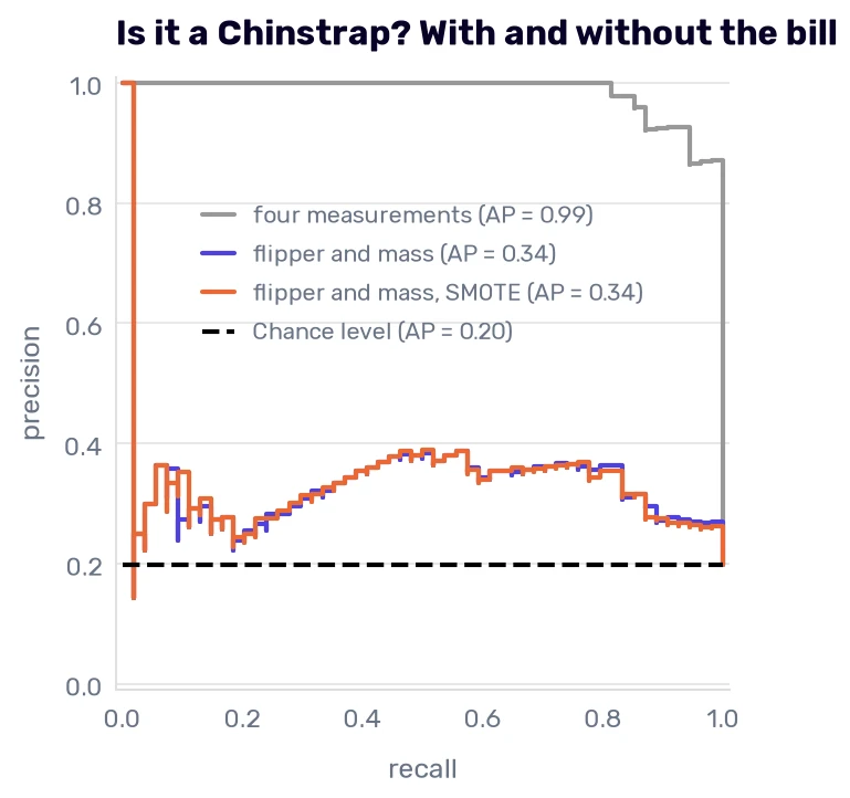
The two lower curves are the model with and without SMOTE, and you can hardly tell them apart. Both run just above the dashed line, the 0.198 that random guessing gets. (The curve is defined to start at a precision of 1 at a recall of 0. The vertical line joins that made-up point to the first real one, which is low because the penguins the model is surest about aren’t Chinstraps.) The gray curve at the top is the model that has the bill.
The resampled models didn’t learn where the Chinstraps are. They say “Chinstrap” far more often and are right at about the same rate. Their scores average 0.44 to 0.46, in a table where 19.8% of the penguins are Chinstraps.
Resampling changes how many rows of each class the model sees. The columns stay what they were. Rule 16 said that when the information is missing, we should stop transforming and go collect it, and a resampler is one more transformation. Two bill measurements took the average precision from 0.34 to 0.99. No sampler in this chapter moved it by more than 0.01 in the right direction.
When the class is really rare
Our classes are 4 to 1. What happens at 35 to 1?
We can simulate it without touching the data file. In every fold, the training part keeps only a few Chinstraps, drawn at random, and the validation part keeps all of its penguins, so we still have 54 Chinstraps to count. A real rare class wouldn’t be that generous: the validation data would be as thin as the training data, and with one or two positives per fold every number in this chapter would jump around. Take the following as a laboratory setup.
from imblearn.ensemble import BalancedRandomForestClassifier
from sklearn.model_selection import FixedThresholdClassifier

def thinned(model, chinstraps_kept, repeats=10):
    rng = np.random.default_rng(42)
    draws = []
    for _ in range(repeats):
        said = np.zeros(len(train_df), dtype=bool)
        share = np.zeros(len(train_df))
        for train_rows, validation_rows in folds.split(train_df, is_chinstrap):
            chinstraps = train_rows[is_chinstrap[train_rows]]
            others = train_rows[~is_chinstrap[train_rows]]
            rows = np.concatenate([others, rng.choice(chinstraps, chinstraps_kept, replace=False)])
            fitted = clone(model).fit(train_df[numeric].iloc[rows], is_chinstrap[rows])
            said[validation_rows] = fitted.predict(train_df[numeric].iloc[validation_rows])
            share[validation_rows] = fitted.predict_proba(train_df[numeric].iloc[validation_rows])[:, 1]
        draws.append({
            'found': (said & is_chinstrap).sum(),
            'false alarms': (said & ~is_chinstrap).sum(),
            'average precision': average_precision_score(is_chinstrap, share),
        })
    return pd.DataFrame(draws).mean()

thin = {}
for chinstraps_kept in [40, 20, 10, 5]:
    share_kept = chinstraps_kept / (chinstraps_kept + 175)
    candidates = {
        'logistic regression': logistic,
        'with a lower threshold': FixedThresholdClassifier(logistic, threshold=share_kept),
        'with class weights': weighted,
        'with random oversampling': resampled(RandomOverSampler(random_state=42), LogisticRegression()),
        'with SMOTE': resampled(SMOTE(k_neighbors=3, random_state=42), LogisticRegression()),
        'with random undersampling': resampled(RandomUnderSampler(random_state=42), LogisticRegression()),
        'forest': RandomForestClassifier(random_state=42),
        'forest with class weights': RandomForestClassifier(class_weight='balanced', random_state=42),
        'forest with a lower threshold': FixedThresholdClassifier(RandomForestClassifier(random_state=42), threshold=share_kept),
        'balanced forest': BalancedRandomForestClassifier(random_state=42),
    }
    thin[chinstraps_kept] = pd.DataFrame({name: thinned(model, chinstraps_kept) for name, model in candidates.items()}).T

pd.DataFrame({kept: table['found'] for kept, table in thin.items()}).rename_axis('Chinstraps kept', axis=1)
| 40 | 20 | 10 | 5 | |
|---|---|---|---|---|
| logistic regression | 46.9 | 40.2 | 31.2 | 19.4 |
| with a lower threshold | 54 | 53.9 | 53.5 | 53.6 |
| with class weights | 52.8 | 51.9 | 51.1 | 49.5 |
| with random oversampling | 52.6 | 51.7 | 50.8 | 49.4 |
| with SMOTE | 51.9 | 50.5 | 49.5 | 48.5 |
| with random undersampling | 52.6 | 50.9 | 49.7 | 48.9 |
| forest | 47.5 | 41.6 | 35.1 | 21.9 |
| forest with class weights | 50.1 | 47.7 | 41.8 | 31.3 |
| forest with a lower threshold | 53 | 52.2 | 50.8 | 48.3 |
| balanced forest | 51.3 | 49.3 | 48.1 | 43.9 |
The table counts the Chinstraps found, out of 54, as an average of 10 draws. Each column is the number of Chinstraps left in every training part, next to about 175 other penguins.
With 40 Chinstraps, we are close to where we have been all chapter (the folds had 43 or 44). Then the untouched logistic regression falls apart. It finds 40 Chinstraps when it has 20 to learn from, 31 when it has 10, and 19 when it has 5. At that point, the Chinstraps are 2.8% of the training part, and the model misses almost two thirds of them.
Class weights and random oversampling hold at 49 or 50 of 54. At full size, the weights were worth 6 Chinstraps, and here they are worth 30.
The forest behaves differently. Class weights take it from 22 to 31, far short of what they do for the logistic regression. Here is every number for the hardest column:
thin[5].round(3)
| found | false alarms | average precision | |
|---|---|---|---|
| logistic regression | 19.4 | 0 | 0.97 |
| with a lower threshold | 53.6 | 32.9 | 0.97 |
| with class weights | 49.5 | 5.9 | 0.975 |
| with random oversampling | 49.4 | 5.5 | 0.976 |
| with SMOTE | 48.5 | 4.4 | 0.977 |
| with random undersampling | 48.9 | 42.1 | 0.683 |
| forest | 21.9 | 0 | 0.909 |
| forest with class weights | 31.3 | 0.8 | 0.905 |
| forest with a lower threshold | 48.3 | 18.8 | 0.909 |
| balanced forest | 43.9 | 3.7 | 0.911 |
Start with the last column. With five Chinstraps to learn from, the untouched logistic regression has an average precision of 0.970, and the weighted one has 0.975. The untouched model still ranks the penguins almost as well. It has learned that a Chinstrap is 1 penguin in 36, so hardly anything gets a score above 0.5, which makes this the threshold problem again.
The second row moves the threshold to the Chinstraps’ share of the training part (0.028 with five kept), which is the arithmetic from It was the threshold. It finds nearly all 54, and it overshoots with 33 false alarms where the weights raise 6. That gap is far more than coefficients moving a little, and the default penalty is involved. With the penalty a million times weaker (C=1e6), the gap is gone: the computed threshold finds 48 Chinstraps with 4 false alarms, and the weights find 46 with 3. Most of the threshold’s job is gone too, because that model finds 44 at a plain 0.5. Its scores sit near 0 and 1, so it matters little where they get cut. I can say that with five positives the default penalty is what holds the untouched model down, and this table doesn’t tell me more than that. A computed threshold is a starting point, and the one you use still gets chosen on validation data.
SMOTE does no better than the copies. With five Chinstraps, every synthetic one lies between two of the five. (I set k_neighbors=3, because the default of five neighbors needs at least six Chinstraps and raises an error with fewer.)
Random undersampling keeps 5 other penguins to match the 5 Chinstraps, and a model trained on 10 penguins raises 42 false alarms. Its average precision drops to 0.68, the lowest in the table.
The forest’s problem is in the last column too. Its average precision is 0.91 in all four forest rows, down from about 0.98 with 40 Chinstraps, so its ranking suffers from the thinning in a way the logistic regression’s doesn’t. The weights can’t repair that. Since scikit-learn 1.9, the forest uses the weights to draw each tree’s bootstrap sample, so with 'balanced' every tree sees about as many Chinstrap rows as other rows, all of them copies of the same five. That buys 9 Chinstraps and no better ranking. class_weight='balanced_subsample' draws the usual sample first and weights it afterwards. Then the weights only change which splits get chosen, a fully grown tree still ends in pure leaves, a pure leaf gives the same answer under any weights, and the count is the plain forest’s 22.
What the forest can still use is the threshold. With the computed one, it finds 48 Chinstraps with 19 false alarms. Imbalanced-learn’s BalancedRandomForestClassifier, which undersamples the common class separately for every tree, finds 44 with 4.
No look at the test set
Nothing in this chapter changed the model we chose. With weights or with SMOTE, the three-species logistic regression went from 269 to 270, a tie of one penguin. It stays as it was, and there is no reason to spend a look at the test set on it (Rule 14).
If you take one habit from the Chinstrap question, make it the order of the attempts. Decide first what a missed positive and a false alarm cost. Then try a threshold chosen on validation data, then class weights, and after those a sampler inside the pipeline. Compare them by the counts and by the average precision, which tells you whether a method did more than move your threshold. The order flips when the positives are very scarce. With one or two of them in a validation fold, there is nothing to tune a threshold on, and the threshold computed from the class share overshot in the table above. Class weights held up there without any tuning, so they come first. They fix the trade at the class ratio, so check it against your costs as soon as you have the positives to do it.
And when the average precision is low and nothing moves it, the model is missing columns, as the one without the bill was. In the next chapter, we look at the columns again and ask which of them a model needs.