
Every group of penguins in this book came from a column. Somebody on the expedition looked at each bird and wrote down a species, and we have used that word ever since. What if nobody had? Suppose the table held only the four measurements. Would it still tell us that it contains three kinds of penguins?
Finding groups without a column that names them is called clustering. I will show you two algorithms, KMeans and DBSCAN, on the 273 training penguins. We happen to know the species, so we can do something you usually can’t: check the groups against an answer the algorithm never saw. At the end, one of the two goes back to the cars, where I owe you a number.
KMeans
KMeans wants one thing from us in advance, the number of groups. We ask for three. It picks three points as centers, gives every penguin to its nearest center, moves each center to the average of the penguins it got, and repeats the last two steps until no penguin changes sides. “Nearest” is a distance, so the columns are scaled first, like for the nearest neighbors.
from sklearn.cluster import KMeans

scaled = StandardScaler().fit_transform(train_df[numeric])
groups = KMeans(n_clusters=3, n_init=10, random_state=42).fit(scaled)
pd.crosstab(groups.labels_, species, rownames=['group'])
| group | Adelie | Chinstrap | Gentoo |
|---|---|---|---|
| 0 | 18 | 49 | 0 |
| 1 | 0 | 0 | 98 |
| 2 | 103 | 5 | 0 |
The group numbers mean nothing (with another seed, the same groups come back numbered differently). To count how well the groups match the species, I pair every group with one species so that as many penguins as possible agree:
from scipy.optimize import linear_sum_assignment

def agreement(labels, other=species):
    table = pd.crosstab(labels, other).values
    return int(table[linear_sum_assignment(-table)].sum())

agreement(groups.labels_)
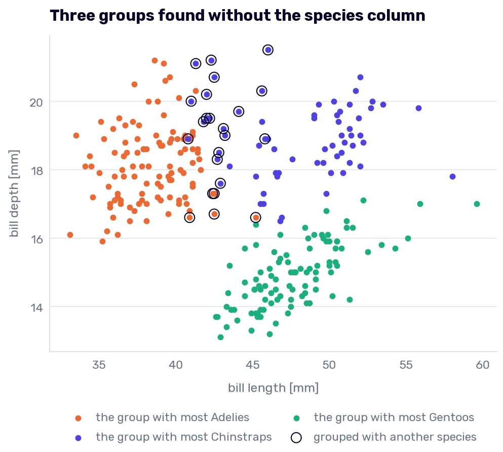
250 of 273. (The usual measure is the adjusted Rand index, adjusted_rand_score in scikit-learn. It needs no pairing, and it’s harder to read than a count of penguins.) The classifier from Hyperparameter search gets about 269 right, but it had the species column to learn from. KMeans got four columns of numbers and found every Gentoo.
The other 23 penguins sit in the group of the wrong species. Who are they?
names = pd.crosstab(groups.labels_, species).idxmax(axis=1)
guess = pd.Series(groups.labels_, index=train_df.index).map(names)
other_side = train_df[guess != species.astype(str)]
pd.crosstab(other_side['species'].astype(str), other_side['sex'])
| species | FEMALE | MALE |
|---|---|---|
| Adelie | 0 | 18 |
| Chinstrap | 5 | 0 |
They are 18 Adelie males and 5 Chinstrap females. Rows 172 and 182 are among them, the two penguins that every model in The penguins they get wrong missed. A big Adelie male and a small Chinstrap female overlap in these four columns, and they did before any model tried to draw a border between them.
fig, ax = plt.subplots(figsize=(7.6, 5.4))
for name, color in SPECIES_COLORS.items():
    members = train_df[guess == name]
    ax.scatter(members['culmen_length_mm'], members['culmen_depth_mm'], color=color, s=22, label=f'the group with most {name}s')
ax.scatter(other_side['culmen_length_mm'], other_side['culmen_depth_mm'], facecolors='none', edgecolors='#080227', s=90, label='grouped with another species')
ax.set_xlabel('bill length [mm]')
ax.set_ylabel('bill depth [mm]')
ax.set_title('Three groups found without the species column', loc='left')
ax.legend(loc='upper center', bbox_to_anchor=(0.5, -0.16), ncol=2)
plt.show()
Where it starts
I passed n_init=10 above without a word. The first three centers are drawn at random (by a method called k-means++, which spreads them out), and where KMeans ends depends on where it starts. By default, it starts once. Here are 100 seeds with the default:
starts = pd.DataFrame([
    {'inertia': round(model.inertia_), 'agreement': agreement(model.labels_)}
    for model in (KMeans(n_clusters=3, random_state=seed).fit(scaled) for seed in range(100))
])
starts.groupby('inertia')['agreement'].agg(['count', 'min', 'max'])
| inertia | count | min | max |
|---|---|---|---|
| 293 | 54 | 250 | 250 |
| 296 | 29 | 260 | 262 |
| 386 | 8 | 172 | 173 |
| 387 | 9 | 176 | 179 |
The inertia is the number KMeans tries to make small: the sum of squared distances between every penguin and the center of its group. About half of the starts end at 293, 29 end a little higher, and 17 end somewhere else entirely. Here is one of the 17:
species_and_sex = species.astype(str) + ' ' + train_df['sex'].str.lower()
unlucky = KMeans(n_clusters=3, random_state=3).fit(scaled)
pd.crosstab(species_and_sex.rename('group'), unlucky.labels_)
| group | 0 | 1 | 2 |
|---|---|---|---|
| Adelie female | 0 | 61 | 0 |
| Adelie male | 0 | 60 | 0 |
| Chinstrap female | 0 | 26 | 0 |
| Chinstrap male | 1 | 27 | 0 |
| Gentoo female | 2 | 0 | 48 |
| Gentoo male | 45 | 0 | 3 |
All the Adelies and Chinstraps share one group, and the Gentoos are split into females and males. Those are three groups too, and one run in six returns them with no warning.
With n_init=10, KMeans starts 10 times and keeps the result with the lowest inertia, which protects us from the last two rows. Now look at the first two. The lowest inertia agrees with the species on 250 penguins, and the second lowest on 260 to 262. By the algorithm’s own measure, the better result is the worse match. KMeans makes distances small. It has never heard of a species, and nothing in the inertia says which of the two results we wanted.
What “similar” means
The columns we hand over decide what a group is. Here are three groups again, asked for three times: on the scaled columns, on the raw ones, and on the scaled columns without the body mass.
def kmeans_agreement(table):
    return agreement(KMeans(n_clusters=3, n_init=10, random_state=42).fit(table).labels_)

pd.Series({
    'scaled': kmeans_agreement(scaled),
    'not scaled': kmeans_agreement(train_df[numeric]),
    'scaled, without the body mass': kmeans_agreement(scaled[:, :3]),
})
| 0 | |
|---|---|
| scaled | 250 |
| not scaled | 164 |
| scaled, without the body mass | 265 |
Without the scaler, the grams drown the millimeters, the way the pounds did in What the scaler decides:
(train_df[numeric].var() / train_df[numeric].var().sum()).round(4)
| 0 | |
|---|---|
| culmen_length_mm | 0 |
| culmen_depth_mm | 0 |
| flipper_length_mm | 0.0003 |
| body_mass_g | 0.9996 |
The body mass is 99.96% of the variance of the raw columns, so KMeans sorts the penguins into three weight classes.
The third row is the interesting one. Dropping a column made the groups match the species better, by 15 penguins. In Males and females, the males of every species were heavier by 435 to 824 g. The body mass separates the sexes as much as the species, and KMeans can’t know which of the two we care about.
KMeans also has an opinion of its own about what a group looks like. It measures distance the same way in every direction, so the border between two groups is a flat wall halfway between their centers, whichever way the groups are stretched. The penguins of one species are stretched along their size, because a big bird has a longer bill, longer flippers, and more mass all at once. The usual next step is a Gaussian mixture, which gives every group its own stretched shape:
from sklearn.mixture import GaussianMixture

mixture = GaussianMixture(n_components=3, n_init=10, random_state=0).fit(scaled)
agreement(mixture.predict(scaled))
268
The mixture matches the species on 268 of 273 penguins, on all four scaled columns, one penguin short of the classifier and still without the species column. I won’t go into mixtures in this book. The point is the 18 penguins between 250 and 268: KMeans lost them to the shape it assumes, and no setting of KMeans would have told us.
How many groups?
I asked for three groups because I knew there were three species. Without the species column, I wouldn’t have known. The inertia can’t choose for us, because it falls with every group we add. The usual tool is the silhouette score. For every penguin, take \(a\), its average distance to the penguins of its own group, and \(b\), its average distance to the penguins of the nearest other group:
\[s = \frac{b - a}{\max(a, b)}\]A penguin deep inside a group that is far from the others gets a score near 1. A penguin between two groups gets a score near 0, and a negative score means it’s closer to the neighbors’ group than to its own. The score of a clustering is the average over all penguins.
from sklearn.metrics import silhouette_score

rows = {}
for k in range(2, 7):
    model = KMeans(n_clusters=k, n_init=10, random_state=42).fit(scaled)
    rows[k] = {'inertia': model.inertia_, 'silhouette': silhouette_score(scaled, model.labels_)}

pd.DataFrame(rows).T.round({'inertia': 0, 'silhouette': 3})
| inertia | silhouette | |
|---|---|---|
| 2 | 448 | 0.534 |
| 3 | 293 | 0.459 |
| 4 | 232 | 0.409 |
| 5 | 178 | 0.388 |
| 6 | 158 | 0.373 |
The silhouette says two. Those two groups are the Gentoos and everybody else, the two peaks from The flipper has two peaks. Three, the number we know to be right, comes second. And if we keep going?
six = KMeans(n_clusters=6, n_init=10, random_state=42).fit(scaled)
pd.crosstab(species_and_sex.rename('group'), six.labels_)
| group | 0 | 1 | 2 | 3 | 4 | 5 |
|---|---|---|---|---|---|---|
| Adelie female | 60 | 0 | 0 | 1 | 0 | 0 |
| Adelie male | 14 | 0 | 0 | 44 | 0 | 2 |
| Chinstrap female | 4 | 0 | 2 | 0 | 0 | 20 |
| Chinstrap male | 0 | 0 | 25 | 0 | 0 | 3 |
| Gentoo female | 0 | 48 | 0 | 0 | 2 | 0 |
| Gentoo male | 0 | 3 | 0 | 0 | 45 | 0 |
Every species has a group that is mostly its females and a group that is mostly its males. With six groups, KMeans found the sexes (with four, it splits only the Gentoos, and with five, the Adelies too).
Two groups, three, and six are all true descriptions of these penguins: the Gentoos and the rest, the species, the species and the sexes. The score ranks them by how far apart the groups sit, and how useful they are is a different question. I used the silhouette score to choose the number of topics in my article about topic modeling with word embeddings. It chose three topics for the articles on my blog, and the fourth group, one step past the best score, was a real topic too (AWS, I used to write a lot about AWS). The number of groups is a decision about what you need the groups for, and the score is one input to it.
Groups made of nothing
Here is a table with no groups in it. Its 273 rows are random numbers drawn from one cloud, and the cloud has the same correlations between its four columns as the scaled penguins have:
one_cloud = np.random.default_rng(0).multivariate_normal(np.zeros(4), np.cov(scaled.T), size=273)
made_up = KMeans(n_clusters=3, n_init=10, random_state=42).fit(one_cloud)
np.bincount(made_up.labels_), round(silhouette_score(one_cloud, made_up.labels_), 3)
(array([ 84, 67, 122]), 0.275)
Three groups of 84, 67, and 122 rows. We asked for three, and KMeans delivered. The silhouette of 0.275 is lower than the penguins’ 0.459, but nothing in the output says how low is too low.
If the groups are real, they should come back when the rows change a little. I draw 273 rows at random from the table (with repeats, so some rows are drawn twice and some are left out), fit KMeans, and do it again with a second draw. Then both models assign all 273 rows, and I count the rows that got the same group from both. The function repeats this 20 times and returns the median:
def comes_back(table, k, repeats=20):
    rng = np.random.default_rng(1)
    same = []
    for _ in range(repeats):
        first, second = (
            KMeans(n_clusters=k, n_init=10, random_state=0).fit(table[rng.choice(len(table), len(table))]).predict(table)
            for _ in range(2)
        )
        same.append(agreement(first, second))
    return int(np.median(same))

pd.DataFrame({
    'penguins': {k: comes_back(scaled, k) for k in (2, 3, 4)},
    'one cloud': {k: comes_back(one_cloud, k) for k in (2, 3, 4)},
}).rename_axis('groups')
| groups | penguins | one cloud |
|---|---|---|
| 2 | 273 | 271 |
| 3 | 264 | 232 |
| 4 | 248 | 208 |
With two groups, the two models agree on every penguin. They also agree on 271 rows of the cloud, where there is nothing to find. A stretched cloud gets cut in half across its long side, and the cut lands in the same place in every draw. So the two groups of penguins pass a check that a table without groups passes too, and it can’t tell them apart. (The gap between the Gentoos and the rest is real. We will measure it in the next section.)
With three groups, 9 penguins change sides against 41 rows of the cloud, and with four, 25 against 65. The penguins’ groups come back more often than the groups of a table that has none, which is the most this check can say. It works the way the noise columns did in Noise as a yardstick: a count like 264 means nothing until the same count from random numbers stands next to it. Groups that fail the comparison aren’t there. Groups that pass it have only passed a filter.
DBSCAN
KMeans needs the number of groups, and every penguin has to join one. DBSCAN asks a different question: where are the penguins crowded together? It takes a distance, eps, and a count, min_samples. A penguin with at least min_samples penguins within eps of it (itself included) is a core point. Core points within eps of each other belong to the same group, and so does any penguin within eps of a core point. Everybody else is noise and gets the label −1.
from sklearn.cluster import DBSCAN

dense = DBSCAN(eps=0.8, min_samples=5).fit(scaled)
pd.crosstab(dense.labels_, species, rownames=['group'])
| group | Adelie | Chinstrap | Gentoo |
|---|---|---|---|
| -1 | 0 | 1 | 3 |
| 0 | 121 | 53 | 0 |
| 1 | 0 | 0 | 95 |
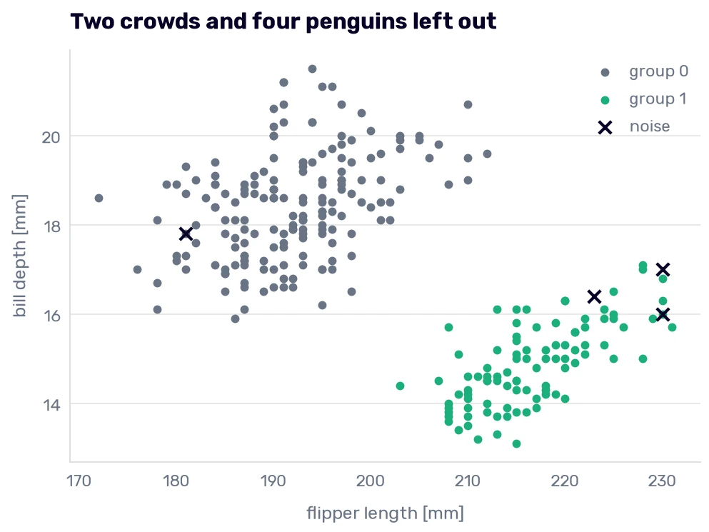
We never said how many groups we wanted, and DBSCAN found two: 121 Adelies with 53 Chinstraps, and 95 Gentoos. Four penguins are noise. It’s the Gentoos and everybody else again. Why can’t it tell an Adelie from a Chinstrap?
from sklearn.metrics import pairwise_distances

is_gentoo = (species == 'Gentoo').values
is_adelie = (species == 'Adelie').values
is_chinstrap = (species == 'Chinstrap').values
pd.Series({
    'from a Gentoo to the nearest other penguin': pairwise_distances(scaled[is_gentoo], scaled[~is_gentoo]).min(),
    'from an Adelie to the nearest Chinstrap': pairwise_distances(scaled[is_adelie], scaled[is_chinstrap]).min(),
}).round(2)
| 0 | |
|---|---|
| from a Gentoo to the nearest other penguin | 1.71 |
| from an Adelie to the nearest Chinstrap | 0.15 |
The Gentoos live across a gap. No Gentoo has a penguin of another species within 1.71, so any eps below that keeps them apart. An Adelie and a Chinstrap sit 0.15 from each other (they are rows 73 and 160, the near-twins from Cleaning the border). A chain of close neighbors leads from one species into the other, and DBSCAN follows chains. An eps small enough to cut this one leaves a quarter of the penguins outside every group, as the next table shows.
fig, ax = plt.subplots(figsize=(7.6, 5))
for label, color in [(0, '#687385'), (1, SPECIES_COLORS['Gentoo'])]:
    members = train_df[dense.labels_ == label]
    ax.scatter(members['flipper_length_mm'], members['culmen_depth_mm'], color=color, s=22, label=f'group {label}')
left_out = train_df[dense.labels_ == -1]
ax.scatter(left_out['flipper_length_mm'], left_out['culmen_depth_mm'], color='#080227', marker='x', s=70, label='noise')
ax.set_xlabel('flipper length [mm]')
ax.set_ylabel('bill depth [mm]')
ax.set_title('Two crowds and four penguins left out', loc='left')
ax.legend()
plt.show()
The settings matter as much as the number of groups did for KMeans:
rows = {}
for eps in (0.5, 0.8, 1.0):
    labels = DBSCAN(eps=eps, min_samples=5).fit(scaled).labels_
    rows[eps] = {'groups': labels.max() + 1, 'noise': (labels == -1).sum()}

pd.DataFrame(rows).T.rename_axis('eps')
| eps | groups | noise |
|---|---|---|
| 0.5 | 4 | 70 |
| 0.8 | 2 | 4 |
| 1 | 2 | 1 |
At 0.5, the crowd breaks into four groups, and 70 penguins belong to none. (The usual advice for choosing eps is to sort the penguins by the distance to their fourth-nearest neighbor and put eps where that distance starts to climb.) At 1.0, one penguin is left out:
train_df[DBSCAN(eps=1.0, min_samples=5).fit(scaled).labels_ == -1][numeric + ['species', 'sex']]
| culmen_length_mm | culmen_depth_mm | flipper_length_mm | body_mass_g | species | sex | |
|---|---|---|---|---|---|---|
| 169 | 58 | 17.8 | 181 | 3700 | Chinstrap | FEMALE |
Row 169 is a Chinstrap female with a 58-millimeter bill, the longest of any Chinstrap in the training data, on a short flipper. Finding the rows that belong to no crowd is half of what DBSCAN gets used for. Rule 1 sends us to the raw file for a row like this:
raw[raw['nest'] == raw.loc[169, 'nest']][['Sex', 'Culmen Length (mm)', 'Flipper Length (mm)', 'Body Mass (g)', 'Comments']]
| Sex | Culmen Length (mm) | Flipper Length (mm) | Body Mass (g) | Comments | |
|---|---|---|---|---|---|
| 168 | MALE | 50.3 | 197 | 3300 | Nest never observed with full clutch. |
| 169 | FEMALE | 58 | 181 | 3700 | Nest never observed with full clutch. |
The file doesn’t question the measurement. It does show that she is 400 g heavier than her mate, with a bill 7.7 mm longer than his, in a species where the male is the bigger bird. The sex came from a blood sample, and the flippers fit it (his is the longer one). So either she is an unusual female, or a bill length or a mass was written down next to the wrong bird. I can’t tell which from here, and I would ask the people who measured her before training anything that depends on her.
Two more differences from KMeans. DBSCAN has no predict, so a new penguin can’t be given a group without running everything again. And it needs the scaler just as much. With the default settings on the raw columns, every penguin is noise:
(DBSCAN().fit(train_df[numeric]).labels_ == -1).sum()
273
Back to the cars
In Regression evaluation metrics, I said that the ceiling for our regressor is set by cars with similar features and different MPG, and a footnote admitted that we didn’t know how many of them we had. Now we can count them.
DBSCAN is the tool for it. A look-alike is a car with another car very close to it. We don’t know how many groups to expect, and most cars should end up in none. So a group may be as small as two cars, and eps is a tenth of a standard deviation (88 lbs, if the weight were the only difference). The cars are the 1970-1979 ones we trained on:
cars = pd.read_csv(data_url, sep=r"\s+", names=column_names, na_values="?").dropna()
cars = cars[cars['model year'] <= 79]
specs = ['cylinders', 'displacement', 'horsepower', 'weight', 'acceleration']

alike = DBSCAN(eps=0.1, min_samples=2).fit(StandardScaler().fit_transform(cars[specs]))
look_alikes = cars.assign(group=alike.labels_)[alike.labels_ >= 0]
len(look_alikes), look_alikes['group'].nunique()
(38, 18)
Of the 307 cars, 38 have a look-alike, in 18 groups. One of them is familiar from Train-test split:
look_alikes[look_alikes['group'] == look_alikes.loc[99, 'group']][specs + ['model year', 'car name', 'mpg']]
| cylinders | displacement | horsepower | weight | acceleration | model year | car name | mpg | |
|---|---|---|---|---|---|---|---|---|
| 99 | 6 | 232 | 100 | 2945 | 16 | 73 | amc hornet | 18 |
| 127 | 6 | 232 | 100 | 2901 | 16 | 74 | amc hornet | 19 |
| 169 | 6 | 232 | 100 | 2914 | 16 | 75 | amc gremlin | 20 |
Two Hornets and a Gremlin, 18, 19, and 20 mpg. How far apart is the MPG inside the groups?
off_group_mean = look_alikes['mpg'] - look_alikes.groupby('group')['mpg'].transform('mean')
round(float(np.sqrt((off_group_mean ** 2).sum() / (len(look_alikes) - look_alikes['group'].nunique()))), 2)
1.85
The standard deviation inside the groups is 1.85 mpg (the division by cars minus groups pays for the 18 group means we estimated). A model that sees only these five columns can’t tell the cars of a group apart, so on such cars its RMSE can’t go much below 1.85. Our best year-blind models scored about 3.1 on the folds, and the model we shipped in The year comes back scored 2.59.
Three cautions, because Rule 10 deserves an honest ceiling. The cars of a group usually come from different years, so the year explains part of the 1.85, and the shipped model knows the year. The estimate is rough: 38 cars in 18 groups leave 20 differences to estimate from, and a spread of 1.4 or of 2.7 would fit them about as well. And I chose eps. At 0.2, DBSCAN starts chaining: one group grows to 16 cars between 1915 and 2300 lbs, where every car has a close neighbor and the two ends are not look-alikes at all.
Nobody had looked
We could check every group in this chapter against the species column. Most groups people work with were never checked against anything.
I remember a strategic initiative for high-value locations. It was a board-level project with dashboards for the C-level, and it kept several teams busy: product, engineering, user-generated content, and marketing. All of it rested on one premise. Those locations were hotels by the sea, beach destinations, and that assumption decided the audience targeting, the UX, and the advertising.
Nobody had plotted the hotels on a map, so I did. It took five minutes in a notebook. The hotels were everywhere: in the mountains, in cities, and by the sea too, obviously. I talked with the product team, and we cut about 40% of the locations. After that, the metric the board was watching started to mean something.
Four teams and a board-level initiative had been built on a group that five minutes of looking took apart. Nobody was lazy. The assumption was old and confident, it felt true, and at that point in the project, looking wasn’t anybody’s job.
I find summaries cringe, and I’m terrible at farewells, so let’s skip both. Go look at some data instead.