
Feature selection ended on a list of settings I had picked by hand: six columns for the filter, a C of 0.1 for the selector, five neighbors because five is the default. I promised that a search inside the folds could choose them.
We have run such a search once. In Choosing alpha, GridSearchCV tried 44 combinations of a polynomial degree and a penalty on the cars. The winner led by 0.04 mpg, lost the last year, and we kept the old pipeline. That chapter also gave us the word hyperparameter (a value we choose before fit() runs) and Rule 19, which said that the best score of a search flatters the winner.
So you know what a grid search is. This chapter is about three things you don’t know yet: how to search when a grid gets too big, what Optuna does differently, and how to tell whether a search found anything. On the penguins, the third question takes the most space.
Here are the settings worth searching for the models in this book. Every other argument of these classes can stay at its default until you have a reason:
| Model | Settings worth a search | What they trade |
|---|---|---|
| Nearest neighbors |
n_neighbors, weights, the distance |
A small k follows single penguins, a large k averages over a crowd |
| Logistic regression | C |
Small coefficients against confident probabilities |
| Decision tree | min_samples_leaf |
How many rows stand behind an answer |
| Random forest |
max_features, min_samples_leaf
|
How different the trees are from each other |
| Boosting |
learning_rate with max_iter, the tree size, the penalty |
Many careful steps against a few big ones |
How far does the score move when nothing changes?
Since The first classifiers and their mistakes, I have called a difference of one or two penguins a tie. I never measured that. Before we let a search compare hundreds of models by their scores, we should know how much a score moves when the model stays the same.
One thing we can change without touching the model is the shuffle that makes the folds. Our folds come from random_state=42, like every other random choice in this book. Here are 20 other shuffles:
def reshuffled(model, shuffles=20):
    rows = []
    for seed in range(shuffles):
        other_folds = StratifiedKFold(n_splits=5, shuffle=True, random_state=seed)
        shares = cross_val_predict(model, train_df[numeric], species, cv=other_folds, method='predict_proba')
        rows.append({
            'right': (np.unique(species)[shares.argmax(axis=1)] == species).sum(),
            'log loss': log_loss(species, shares),
        })
    return pd.DataFrame(rows)

same_models = {'logistic regression': logistic, 'nearest neighbors': species_knn, 'histogram boosting': hist_boosting}
pd.DataFrame({name: reshuffled(model)['right'].agg(['min', 'mean', 'max']) for name, model in same_models.items()}).T
| min | mean | max | |
|---|---|---|---|
| logistic regression | 267 | 268.7 | 270 |
| nearest neighbors | 267 | 268.2 | 270 |
| histogram boosting | 261 | 264.5 | 267 |
The same logistic regression, with the same settings, on the same 273 penguins, gets anything from 267 to 270. The boosting moves between 261 and 267. Nothing was tuned here. The only thing that changed is which penguins shared a fold.
We can go one step further and search over a setting that can’t matter. A random forest takes a random_state, which decides the bootstrap samples and the columns each split may use. No seed is better than another. Let’s search for the best one anyway:
seeds = pd.Series({
    seed: right(RandomForestClassifier(n_estimators=100, random_state=seed), train_df[numeric])
    for seed in range(30)
})
pd.Series({'lowest': seeds.min(), 'mean': seeds.mean().round(1), 'highest': seeds.max(), 'best seed': seeds.idxmax(), 'worst seed': seeds.idxmin()})
| 0 | |
|---|---|
| lowest | 264 |
| mean | 265.9 |
| highest | 267 |
| best seed | 6 |
| worst seed | 23 |
The best of 30 seeds gets 267 and the worst 264. If the setting had been called max_depth, I would have reported that tuning won three penguins. To see what the winning seed is worth, we give the best and the worst seed the 20 other shuffles:
pd.DataFrame({
    f'seed {seed}': reshuffled(RandomForestClassifier(n_estimators=100, random_state=seed))['right'].agg(['min', 'mean', 'max'])
    for seed in [seeds.idxmax(), seeds.idxmin()]
}).T
| min | mean | max | |
|---|---|---|---|
| seed 6 | 265 | 266.55 | 268 |
| seed 23 | 264 | 266.5 | 269 |
For the logistic regression and the neighbors, that distance is three penguins from the lowest shuffle to the highest. So “one or two penguins is a tie” was about right for them. The boosting moves by six, and a comparison that involves it needs a wider tie.
The grid on the nearest neighbors
Now, the search I promised. The nearest neighbors have three settings worth trying: the number of neighbors, whether a closer neighbor gets a bigger vote (weights='distance'), and how the distance is added up (p=2 is the straight-line distance from the formula, and p=1 sums the absolute differences instead of the squared ones).
from sklearn.model_selection import GridSearchCV

neighbor_grid = {
    'kneighborsclassifier__n_neighbors': [1, 3, 5, 7, 10, 15, 20, 30, 40],
    'kneighborsclassifier__weights': ['uniform', 'distance'],
    'kneighborsclassifier__p': [1, 2],
}
neighbor_search = GridSearchCV(species_knn, neighbor_grid, cv=folds, scoring='balanced_accuracy').fit(train_df[numeric], species)

neighbor_search.best_params_, right(neighbor_search.best_estimator_, train_df[numeric])
({'kneighborsclassifier__n_neighbors': 5, 'kneighborsclassifier__p': 1, 'kneighborsclassifier__weights': 'distance'}, 269)
That’s 9 values times 2 times 2, or 36 combinations. The winner has five neighbors, the other distance, and weighted votes, and it gets 269 penguins right. The default we have used since Nearest neighbors, three species gets 269 too. The search prefers its winner for a balanced accuracy that is 0.4 percentage points higher on average over the folds, because the four mistakes fall on different species. Rule 30 said to ignore a difference of that size.
The search took a second and found the model we already had. A search that confirms the default is a result too: it says the default wasn’t holding the neighbors back, and we can stop wondering.
The settings I picked by hand
The promise was about a longer pipeline: the filter from Filters: every column on its own in front of the neighbors, on the thirty table (the 10 candidate columns and 20 columns of noise). I picked six columns and five neighbors. A grid can pick both at once, because a pipeline’s steps are all open to the search:
selected_neighbors = prepared(SelectKBest(f_classif), KNeighborsClassifier())
thirty_grid = {
    'selectkbest__k': list(range(1, 16)) + [20, 30],
    'kneighborsclassifier__n_neighbors': [1, 3, 5, 10, 20],
}
thirty_search = GridSearchCV(selected_neighbors, thirty_grid, cv=folds, scoring='balanced_accuracy').fit(thirty, species)

thirty_search.best_params_, right(thirty_search.best_estimator_, thirty)
({'kneighborsclassifier__n_neighbors': 1, 'selectkbest__k': 6}, 273)
Six columns and one neighbor get 273 of 273, and so do four other combinations. Don’t believe that number, for two reasons. The thirty table holds the sample number and the egg day (the columns that describe the expedition), and What the model gets threw them out. And the 273 is the best of 85 combinations, scored on the folds that chose it.
Rule 29 said that a choice made with the validation rows’ answers can’t be checked on those rows. The fix is the nested cross-validation we met with RFECV. The whole search becomes the model, and the outer folds score it on penguins that the search never saw:
nested_search = GridSearchCV(selected_neighbors, thirty_grid, cv=inner_folds, scoring='balanced_accuracy')

chosen = [
    clone(nested_search).fit(thirty.iloc[train_rows], species.iloc[train_rows]).best_params_
    for train_rows, _ in folds.split(thirty, species)
]
right(nested_search, thirty), [(choice['selectkbest__k'], choice['kneighborsclassifier__n_neighbors']) for choice in chosen]
(272, [(5, 1), (5, 1), (6, 3), (8, 1), (6, 3)])
The nested score is 272. The five searches chose 5, 5, 6, 8, and 6 columns, with one neighbor or three. So six columns was a reasonable choice to make by hand, and the number of neighbors hardly matters once the noise columns are gone.
What should the search look at?
Both searches had the same weakness. The balanced accuracy is made of counts, and counts take few values, so many combinations share the best score (five shared a perfect one a moment ago). GridSearchCV breaks a tie by taking the combination that comes first in the grid, which is an accident of how I typed it.
The log loss from How it learns, and the log loss doesn’t tie. It moves whenever any probability moves. And we have already seen a search where the two disagreed. In The penalty you didn’t ask for, every C from 1 upward got 269 penguins, and the log loss was 0.060 at the default of 1, 0.032 at 10, and 0.037 at 100. I wrote that I wasn’t switching to 10, because the metric we chose is about the answers.
I’ve changed my mind, and Rule 30 is the reason. Back then, I had one number from one set of folds. Now, we can ask whether the difference survives a reshuffle:
def logistic_with(C):
    return make_pipeline(StandardScaler(), LogisticRegression(C=C, max_iter=10_000))

strengths = {C: reshuffled(logistic_with(C)) for C in [1, 10, 100]}
pd.DataFrame({
    C: {
        'right, lowest': scores['right'].min(),
        'right, mean': scores['right'].mean(),
        'right, highest': scores['right'].max(),
        'log loss, mean': scores['log loss'].mean(),
        'shuffles with a lower log loss than C=1': (scores['log loss'] < strengths[1]['log loss']).sum(),
        'shuffles with a higher count than C=1': (scores['right'] > strengths[1]['right']).sum(),
    }
    for C, scores in strengths.items()
}).T.rename_axis('C').round(3)
| C | right, lowest | right, mean | right, highest | log loss, mean | shuffles with a lower log loss than C=1 | shuffles with a higher count than C=1 |
|---|---|---|---|---|---|---|
| 1 | 267 | 268.7 | 270 | 0.059 | 0 | 0 |
| 10 | 269 | 270.05 | 271 | 0.028 | 20 | 17 |
| 100 | 269 | 269.85 | 271 | 0.024 | 20 | 14 |
C=10 has the lower log loss in all 20 shuffles, and it’s about half: 0.028 against 0.059. It also gets more penguins right in 17 of the 20, with 270.05 on average against 268.7. Our own folds hid that behind a 269 on both sides. A difference of 1.4 penguins is still small, but one that shows up in 17 shuffles of 20 isn’t the kind of movement Rule 30 warned about. Notice that this is a sharper test than comparing two ranges. Both models were scored on the same shuffle each time, so the luck of the split is the same on both sides, and what remains is the difference between the models. Whenever you can compare in pairs like this, do. (The shuffles reuse the penguins that suggested C=10 in the first place, so they aren’t a nested check. With three candidates to choose from, there is little to leak.) C=100 looks as good as 10 in this table, and I will get to it in a moment.
Half the log loss with the same answers means the probabilities got better, and we do use the probabilities. In A second opinion, every penguin with a probability below 0.8 went to somebody who could look at its chin. There were 14 of them, and all four mistakes were among them. Here is that queue for three values of C:
def second_opinions(model, limit=0.8):
    shares = cross_val_predict(model, train_df[numeric], species, cv=folds, method='predict_proba')
    wrong = np.unique(species)[shares.argmax(axis=1)] != species
    unsure = shares.max(axis=1) < limit
    return {
        'right': (~wrong).sum(),
        'log loss': log_loss(species, shares),
        'sent for a second opinion': unsure.sum(),
        'mistakes among them': (wrong & unsure).sum(),
        'mistakes kept': (wrong & ~unsure).sum(),
    }

pd.DataFrame({C: second_opinions(logistic_with(C)) for C in [1, 10, 100]}).T.rename_axis('C').round(3)
| C | right | log loss | sent for a second opinion | mistakes among them | mistakes kept |
|---|---|---|---|---|---|
| 1 | 269 | 0.06 | 14 | 4 | 0 |
| 10 | 269 | 0.032 | 8 | 4 | 0 |
| 100 | 269 | 0.037 | 3 | 1 | 3 |
With C=10, 8 penguins need a second opinion instead of 14, and all four mistakes are still in the queue. Somebody has to catch those birds and look at them, so six fewer is a gain that the count of right answers can’t show.
C=100 shows where it stops. The model is right as often as before and sure about nearly everything. Three penguins fall below 0.8, and three of the four mistakes walk past the check with a high probability. The unpenalized model from The penalty you didn’t ask for is on its way back here: a weak penalty lets the coefficients grow, and bigger coefficients push every probability toward 0 or 1, the wrong ones included.
many_strengths = np.logspace(-1, 3, 13)
by_strength = pd.DataFrame([second_opinions(logistic_with(C)) for C in many_strengths], index=many_strengths)

fig, (top, bottom) = plt.subplots(2, 1, sharex=True, figsize=(7.6, 5.6))
top.plot(by_strength.index, by_strength['log loss'], marker='o')
top.set_ylabel('log loss on the folds')
top.set_title('A weaker penalty makes the model surer, and then too sure', loc='left')
bottom.plot(by_strength.index, by_strength['sent for a second opinion'], marker='o', label='penguins below 0.8')
bottom.plot(by_strength.index, by_strength['mistakes among them'], marker='o', label='mistakes among them')
bottom.set_xscale('log')
bottom.set_xlabel('C (the default is 1)')
bottom.set_ylabel('penguins')
bottom.legend()
plt.show()
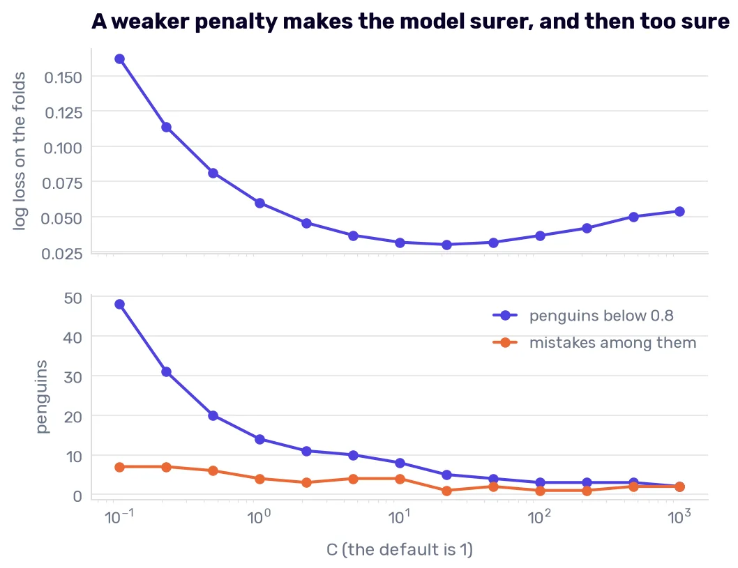
The log loss has a wide, flat bottom between 10 and 50, and its lowest point in this run is at 22. The lower panel has no flat part. Up to a C of 10, every mistake the model makes is in the second-opinion queue. At 22, the queue is down to five penguins, and it holds one of the three mistakes.
So the search needs a number that doesn’t tie, and that number can’t be the only judge. The log loss chose between 10 and 100 by a hair. The table of second opinions made the choice for me, because it shows what the probabilities are used for. I take C=10, and I will come back to it at the end of the chapter.
When the grid gets too big
The logistic regression has one setting, and the neighbors have three. Histogram boosting has five that matter: the learning rate, the number of trees (max_iter), the size of a tree (max_leaf_nodes), the smallest leaf (min_samples_leaf), and a penalty on the leaf values (l2_regularization). It’s also the model with the most to gain. With its defaults, it got 262 penguins, the fewest of our six models, and a log loss of 0.205.
A grid multiplies. With 3 values for each of 5 settings, a grid has 243 combinations, and 3 values are a poor description of a learning rate. With 5 values each, it has 3,125. And most of those fits repeat each other: if the penalty hardly matters, a grid with three penalties trains every other combination three times and learns the same thing three times.
A random search draws every setting at random for every try. With 60 tries, it tests 60 different learning rates and 60 different penalties, and it covers most of the 30 tree sizes. If one setting turns out to be useless, nothing was wasted on it, because the other four still got 60 different values.1
Instead of lists, RandomizedSearchCV takes distributions to draw from:
from scipy.stats import loguniform, randint
from sklearn.model_selection import RandomizedSearchCV

boosting_space = {
    'learning_rate': loguniform(0.01, 1),
    'max_iter': randint(10, 300),
    'max_leaf_nodes': randint(2, 32),
    'min_samples_leaf': randint(1, 41),
    'l2_regularization': loguniform(0.001, 10),
}

def random_search(seed, search_folds=folds):
    return RandomizedSearchCV(
        HistGradientBoostingClassifier(random_state=42), boosting_space,
        n_iter=60, cv=search_folds, scoring='neg_log_loss', random_state=seed, n_jobs=-1,
    )

boosting_grid = {
    'learning_rate': [0.01, 0.1, 1],
    'max_iter': [30, 100, 300],
    'max_leaf_nodes': [4, 16, 31],
    'min_samples_leaf': [5, 20, 40],
}
grid_boosting = GridSearchCV(HistGradientBoostingClassifier(random_state=42), boosting_grid, cv=folds, scoring='neg_log_loss').fit(train_df[numeric], species)
random_boosting = random_search(42).fit(train_df[numeric], species)

pd.DataFrame({
    'the defaults': fold_scores(hist_boosting),
    'grid, 81 combinations': fold_scores(grid_boosting.best_estimator_),
    'random search, 60 draws': fold_scores(random_boosting.best_estimator_),
}).T[['right', 'log loss']].round(3)
| right | log loss | |
|---|---|---|
| the defaults | 262 | 0.205 |
| grid, 81 combinations | 266 | 0.094 |
| random search, 60 draws | 267 | 0.084 |
randint(10, 300) draws whole numbers from 10 to 299. loguniform(0.01, 1) draws a number whose logarithm is uniform, so a learning rate between 0.01 and 0.1 is as likely as one between 0.1 and 1. A plain uniform draw would put 90% of the tries above 0.1. Use loguniform for every setting where you would naturally write the candidates as 0.001, 0.01, 0.1: rates and penalties, C and alpha included. (The scoring is neg_log_loss because scikit-learn’s scorers treat a greater number as better, so the log loss comes back negated.)
Both searches cut the log loss of the defaults by more than half. The random search did a little better than the grid with 60 combinations against 81, and it covered five settings where the grid had four.
Why 60 draws? There is a piece of arithmetic worth remembering. Call the best 5% of all possible combinations “good enough.” One random draw misses that region with a probability of 0.95, and 60 draws all miss it with a probability of 0.95 to the power of 60, which is 5%. So 60 draws land in the best 5% at least once, 95 times out of 100, however many settings there are. A grid fine enough to make the same promise needs far more fits, and the number multiplies with every setting you add.
Now, which settings won?
winners = {}
for seed in range(5):
    search = random_search(seed).fit(train_df[numeric], species)
    winners[seed] = {**search.best_params_, 'log loss': -search.best_score_, 'right': right(search.best_estimator_, train_df[numeric])}

pd.DataFrame(winners).T.rename_axis('search seed').round(3)
| search seed | l2_regularization | learning_rate | max_iter | max_leaf_nodes | min_samples_leaf | log loss | right |
|---|---|---|---|---|---|---|---|
| 0 | 0.006 | 0.055 | 207 | 2 | 37 | 0.085 | 265 |
| 1 | 0.001 | 0.316 | 25 | 2 | 5 | 0.085 | 265 |
| 2 | 1.039 | 0.044 | 166 | 25 | 37 | 0.088 | 264 |
| 3 | 2.274 | 0.284 | 18 | 22 | 9 | 0.085 | 265 |
| 4 | 0.289 | 0.025 | 195 | 24 | 36 | 0.087 | 265 |
Five searches gave five different winners. The learning rate goes from 0.025 to 0.316, the trees have from 2 leaves to 25, and the penalty covers three orders of magnitude. So don’t read a winner’s settings as a fact about the data. “The best learning rate for penguins is 0.055” is a fact about seed 0.
The last column deserves a look too. These five winners get 264 or 265 penguins, and the search with seed 42 claimed 267.
Did the search find anything?
The random search says 267 penguins where the defaults got 262. The boosting moved by six between shuffles on its own, and the 267 is the best of 60 tries, scored on the folds that picked it (Rule 19). So we check it on the reshuffled folds from the start of the chapter.
There is a trap here. The winner was chosen with all 273 penguins. If we score it as a fixed model, every fold validates it on penguins that helped to choose it, which Rule 29 told us never to do. The honest version repeats the whole search inside every training part, as we did with the grid a moment ago. The table has both, and a model with one changed default, max_leaf_nodes=2:
two_leaves = HistGradientBoostingClassifier(random_state=42, max_leaf_nodes=2)

boosting_shuffles = {
    'the defaults': reshuffled(hist_boosting, shuffles=10),
    'the winner, as a fixed model': reshuffled(random_boosting.best_estimator_, shuffles=10),
    'the search, repeated inside every fold': reshuffled(random_search(42, inner_folds), shuffles=10),
    'two leaves': reshuffled(two_leaves, shuffles=10),
}
pd.DataFrame({
    name: {
        'right, mean': scores['right'].mean(),
        'log loss, median': scores['log loss'].median(),
        'log loss, highest': scores['log loss'].max(),
        'shuffles with a lower log loss than the defaults': (scores['log loss'] < boosting_shuffles['the defaults']['log loss']).sum(),
    }
    for name, scores in boosting_shuffles.items()
}).T.round(3)
| right, mean | log loss, median | log loss, highest | shuffles with a lower log loss than the defaults | |
|---|---|---|---|---|
| the defaults | 265 | 0.17 | 0.26 | 0 |
| the winner, as a fixed model | 265.8 | 0.084 | 0.114 | 10 |
| the search, repeated inside every fold | 264.5 | 0.121 | 0.831 | 9 |
| two leaves | 265.4 | 0.088 | 0.111 | 10 |
As a fixed model, the winner halves the defaults’ log loss. Repeated honestly, the search gets no more penguins than the defaults (264.5 against 265.0) and a median log loss of 0.121 against 0.170, and on one shuffle of ten it picked a model that scored 0.831. Most of what the search reported came from the leak, the winner’s curse, and a bad draw of the defaults on our folds (262 against about 265 on average).
The last row beats the search with one changed setting. With max_leaf_nodes=2, every tree asks a single question. I found it by changing one setting at a time before I ran any search, and it comes with a reason I can check. The default boosting gives four of its 11 mistakes on the folds a probability of 1.00, and the log loss charges heavily for a confident mistake. With one question per tree, no mistake gets a 1.00. (The two leaves were chosen with these penguins too, from a handful of tries.)
So before a search, change the settings one at a time. It costs a few fits, and it tells you which settings matter and why. And even with two leaves, the boosting loses to the logistic regression with its default C, which got 269 and 0.060 without any search.
Optuna
A random search doesn’t learn. Its 60th draw knows nothing about the first 59, and if the first 20 tries all said that a learning rate of 1 is hopeless, the 21st may still draw 0.9. Optuna is a library whose default search uses the tries it has already made.
You don’t hand it a grid or a table of distributions. You write a function that gets a trial, asks the trial for a value of each setting, trains whatever you want, and returns a score:
import optuna

optuna.logging.set_verbosity(optuna.logging.WARNING)

def boosting_objective(trial):
    model = HistGradientBoostingClassifier(
        random_state=42,
        learning_rate=trial.suggest_float('learning_rate', 0.01, 1, log=True),
        max_iter=trial.suggest_int('max_iter', 10, 299),
        max_leaf_nodes=trial.suggest_int('max_leaf_nodes', 2, 31),
        min_samples_leaf=trial.suggest_int('min_samples_leaf', 1, 40),
        l2_regularization=trial.suggest_float('l2_regularization', 0.001, 10, log=True),
    )
    return cross_val_score(model, train_df[numeric], species, cv=folds, scoring='neg_log_loss').mean()

def optuna_search(seed, objective=boosting_objective, tries=60):
    study = optuna.create_study(direction='maximize', sampler=optuna.samplers.TPESampler(seed=seed))
    study.optimize(objective, n_trials=tries)
    return study

study = optuna_search(0)
study.best_params, -study.best_value
({'learning_rate': 0.050636476825029524, 'max_iter': 253, 'max_leaf_nodes': 24, 'min_samples_leaf': 7, 'l2_regularization': 3.587893779683567}, 0.0860301679174733)
The space is the one the random search had (log=True is the loguniform, and Optuna’s ranges include both ends). A study is one search, and a trial is one try. direction='maximize' says that a bigger return value is better. Without the seed, every run of the search would try different values.
How it chooses the next try
The sampler is called TPE, the Tree-structured Parzen Estimator, and the idea is simpler than the name.
The first 10 trials are drawn at random, like a random search. From then on, before each trial, the sampler sorts the finished trials by their score and splits them into two groups: the best tenth, and the rest. Then it draws two curves over the values of a setting. One curve shows which values the good trials had, and the other shows which values the rest had. Each curve is a pile of small bumps, one bump per trial, placed at the value that trial used (a histogram with soft edges, if you like).
Now, the sampler needs a value for the next trial. It draws 24 candidates from the curve of the good trials and, for each candidate, divides the height of the good curve by the height of the other curve. A candidate with a high ratio is a value that good trials used often and the others rarely. The candidate with the highest ratio becomes the next trial’s value.
So TPE never predicts the score of a combination. It only asks where the good trials are denser than the others, and it tries there.
One limit follows from the description. “The best tenth” of 20 trials is 2 trials, and two bumps are a thin picture of where the good models are. The sampler needs a few dozen trials before its curves describe anything.
Did learning help on the penguins?
random_runs = {seed: -pd.Series(random_search(seed).fit(train_df[numeric], species).cv_results_['mean_test_score']) for seed in range(3)}
optuna_runs = {seed: -optuna_search(seed).trials_dataframe()['value'] for seed in range(3)}

fig, ax = plt.subplots()
for seed in range(3):
    ax.plot(range(1, 61), random_runs[seed].cummin(), color='C0', label='random search' if seed == 0 else None)
    ax.plot(range(1, 61), optuna_runs[seed].cummin(), color='C1', label='Optuna (TPE)' if seed == 0 else None)
ax.set_xlabel('tries')
ax.set_ylabel('best log loss on the folds so far')
ax.set_ylim(0.08, 0.14)
ax.set_title('Three random searches and three Optuna studies', loc='left')
ax.legend()
plt.show()

pd.DataFrame({
    'random search': [run.cummin().iloc[[9, 19, 59]].tolist() for run in random_runs.values()],
    'Optuna': [run.cummin().iloc[[9, 19, 59]].tolist() for run in optuna_runs.values()],
}).map(lambda best: ' / '.join(f'{value:.3f}' for value in best)).rename_axis('seed')
| seed | random search | Optuna |
|---|---|---|
| 0 | 0.090 / 0.085 / 0.085 | 0.112 / 0.094 / 0.086 |
| 1 | 0.089 / 0.085 / 0.085 | 0.098 / 0.093 / 0.084 |
| 2 | 0.090 / 0.090 / 0.088 | 0.098 / 0.092 / 0.088 |
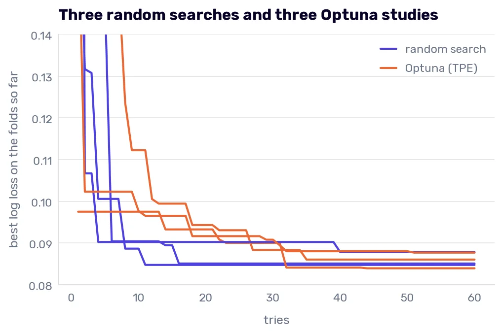
Each cell holds the best log loss after 10, 20, and 60 tries. After 60, the two methods are in the same place: 0.085 to 0.088 for the random search and 0.084 to 0.088 for Optuna. After 10 and 20 tries, Optuna is behind in all three runs. Its first 10 trials are random draws too. They happened to be unluckier ones, and it needed about 30 trials to catch up.
I wouldn’t hold that against Optuna. We have just seen that very different settings of this model all end near 0.085. A sampler that looks for the region where the good trials are has nothing to find when the good trials are everywhere.
A search space with branches
There is one thing the function gives you that a table of distributions can’t. The function is ordinary Python, so a later question can depend on an earlier answer. The kind of model can be a setting, and each model can bring settings of its own:
def model_objective(trial):
    kind = trial.suggest_categorical('model', ['logistic regression', 'nearest neighbors', 'boosting'])
    if kind == 'logistic regression':
        model = logistic_with(trial.suggest_float('C', 0.01, 1000, log=True))
    elif kind == 'nearest neighbors':
        model = make_pipeline(StandardScaler(), KNeighborsClassifier(
            n_neighbors=trial.suggest_int('n_neighbors', 1, 40),
            weights=trial.suggest_categorical('weights', ['uniform', 'distance']),
        ))
    else:
        model = HistGradientBoostingClassifier(
            random_state=42,
            learning_rate=trial.suggest_float('learning_rate', 0.01, 1, log=True),
            max_leaf_nodes=trial.suggest_int('max_leaf_nodes', 2, 31),
        )
    return cross_val_score(model, train_df[numeric], species, cv=folds, scoring='neg_log_loss').mean()

model_study = optuna_search(42, model_objective, tries=100)
trials = model_study.trials_dataframe()

pd.DataFrame({
    'trials': trials.groupby('params_model').size(),
    'best log loss': -trials.groupby('params_model')['value'].max(),
}).rename_axis('model').round(3)
| model | trials | best log loss |
|---|---|---|
| boosting | 9 | 0.109 |
| logistic regression | 79 | 0.03 |
| nearest neighbors | 12 | 0.045 |
model_study.best_params
{'model': 'logistic regression', 'C': 21.5025217028324}
(One detail from How it chooses the next try changes here. A setting that exists in only one branch gets its own pair of curves, unless you pass TPESampler(multivariate=True, group=True).)
Of the 100 trials, 79 went to the logistic regression, 12 to the neighbors, and 9 to the boosting. The sampler saw early which branch had the good scores and spent its tries there, and the winner is the logistic regression with a C of 21.5 and a log loss of 0.030.
Read the other two rows with care. The best boosting in this study has 0.109, and the random search found 0.084. The best neighbors have 0.045, and the default five neighbors get 0.033. A branch that got 9 or 12 trials was barely searched, so the study tells you which model won and very little about how good the losers could have been.
Where Optuna earns its keep
On the penguins, one try takes a tenth of a second, and I can afford to waste 50 of them. The project where I used Optuna at work looked different. The model was a neural network for image recognition, and one training run took about an hour, more or less depending on the number of layers, which was one of the settings we tuned.
We had a Kubernetes cluster for training jobs already, so the search didn’t train anything itself. The function we gave to Optuna set the parameters, started a training job in the cluster by calling kubectl apply from Python, and waited in a loop until the job was done. Nothing fancy. The cluster had three GPU nodes, so three jobs ran at a time. We also wrote the processed results to a cache, so that a process dying in the middle of a run didn’t make us repeat the experiments.
At an hour of a GPU per try, a try spent on a learning rate that 20 earlier tries had already ruled out is an hour gone. At that price, a sampler that reads its own history is worth having, and the other things Optuna offers start to matter: a study can be stored in a database and continued after a crash, several workers can run trials of one study at the same time, and a pruner can stop a trial early when its first results are already worse than those of the trials before it.
(For scikit-learn models, the optuna-integration package has an OptunaSearchCV that looks like RandomizedSearchCV. I wrote the function by hand because the function is the part you will need when the model isn’t a scikit-learn model.)
Searches that cost less
Some settings don’t need a search at all.
The number of boosting rounds is one. With early_stopping=True, the boosting sets aside a tenth of its training rows, watches its score on them, and stops adding trees when the score has not improved for 10 rounds:
early = HistGradientBoostingClassifier(random_state=42, early_stopping=True)
fold_scores(early)[['right', 'log loss']].round(3)
| 0 | |
|---|---|
| right | 263 |
| log loss | 0.107 |
One fit per fold, and the log loss falls from the defaults’ 0.205 to 0.107. (Scikit-learn switches early stopping on by itself when the table has more than 10,000 rows.)
The forest has its out-of-bag score. Every tree is tested on the rows its bootstrap sample left out, so one fit() gives a validation score with no folds, and a loop over a few values of max_features is a search.
For tables too big to fit 60 times, scikit-learn has HalvingGridSearchCV and HalvingRandomSearchCV. They start many candidates on a small sample of the rows, keep the best third, give the survivors three times as many rows, and repeat. Our 273 penguins are the wrong place to show them: the first round would train on 30 birds.
What a search can’t find
A search looks only inside the space you gave it. In Why not keep everything?, 20 columns of noise took the nearest neighbors from 269 to 241, and 500 took the logistic regression to 214. Can the right k or the right C win those penguins back?
noisy = train_df[numeric].join(noise.iloc[:, :20])
noisiest = train_df[numeric].join(noise)

pd.Series({k: right(make_pipeline(StandardScaler(), KNeighborsClassifier(n_neighbors=k)), noisy) for k in [1, 3, 5, 10, 20, 40, 80]}, name='right, of 273').rename_axis('k').to_frame().T
| 1 | 3 | 5 | 10 | 20 | 40 | 80 | |
|---|---|---|---|---|---|---|---|
| right, of 273 | 228 | 238 | 241 | 243 | 233 | 229 | 220 |
pd.Series({C: right(logistic_with(C), noisiest) for C in [0.001, 0.01, 0.1, 1, 10, 100, 1000]}, name='right, of 273').rename_axis('C').to_frame().T
| 0.001 | 0.01 | 0.1 | 1.0 | 10.0 | 100.0 | 1000.0 | |
|---|---|---|---|---|---|---|---|
| right, of 273 | 196 | 207 | 216 | 214 | 212 | 208 | 208 |
No. The best k gets 243 where the neighbors without the noise got 269, and the best C gets 216. The search did its job in both cases, in a space that didn’t contain a good model.
Feature selection had one for the second table. An L1 penalty sets coefficients to exactly 0. It takes a different penalty, a solver that supports it, and a C of 0.3 from that chapter’s table:
l1_logistic = make_pipeline(StandardScaler(), LogisticRegression(l1_ratio=1, C=0.3, solver='saga', max_iter=5000, random_state=42))
right(l1_logistic, noisiest)
267
267 with 500 columns of noise in the table. The kind of penalty is a hyperparameter too, and a search would have found it if I had put it into the space. I knew to put it there only because Embedded methods had shown what it does to useless columns. The 20 noise columns in front of the neighbors are a problem for a filter, and no number of neighbors solves it.
This is why choosing the settings is step 8 of the machine learning process, after the features. A search refines a model that is already about right, and the columns decide whether it gets that far.
One look at the test set
This is the last chapter that offers a new species model, and the change is small: the logistic regression on the four scaled measurements, with C=10 where the default was 1.
The test set gave the old model 69 of 69 in One look at the test set, so the count can’t improve. What can improve are the two numbers this chapter was about. I write the expectations down before running the code.
The count: 67 to 69, as before. On the folds, the two models give the same 269 answers in total, so I expect the same 69 here and would shrug at 68.
The log loss: on the folds, C=10 had about half the log loss of C=1 (0.032 against 0.060). I expect it to be lower on the test set too, by a similar share.
The second-opinion queue: two test penguins (rows 37 and 129) were below 0.8 with the old model, and both got the right answer. The queue on the folds shrank from 14 to 8, so I expect one or two here. Row 129 had a probability of 0.51, and I expect it to stay in the queue.
def test_look(C):
    fitted = logistic_with(C).fit(train_df[numeric], species)
    shares = fitted.predict_proba(test_df[numeric])
    return {
        'right, of 69': (fitted.predict(test_df[numeric]) == test_df['species']).sum(),
        'log loss': round(log_loss(test_df['species'], shares), 3),
        'rows below 0.8': test_df.index[shares.max(axis=1) < 0.8].tolist(),
    }

pd.DataFrame({C: test_look(C) for C in [1, 10]}).T.rename_axis('C')
| C | right, of 69 | log loss | rows below 0.8 |
|---|---|---|---|
| 1 | 69 | 0.04 | [37, 129] |
| 10 | 69 | 0.015 | [129] |
Both models get 69 of 69. The log loss fell from 0.040 to 0.015, and the queue went from two penguins to one: row 37 left it, and row 129 is still there. All three expectations held, which doesn’t happen to me often enough to go unmentioned.
Know what this look could and couldn’t show, though. The risk of a weaker penalty is a confident mistake, as C=100 showed on the folds. The test set contains no mistake of this model, so it had no way to show that risk. A lower log loss and a shorter queue on 69 correct answers are what any surer model would produce, C=100 included. The evidence that C=10 doesn’t hide its mistakes is the four of four on the folds, and the test set adds nothing to it.
The caution from the last look applies again. The 69 penguins can agree with the folds, and they can’t prove much beyond that. The number I would report is still the one from the folds: about 269 of 273, with eight penguins sent for a second opinion and all four mistakes among them.
The limit of 0.8 is a setting too. It was chosen for the old model, on the same folds, after seeing where the mistakes were. I kept it here so that the two models could be compared on one line. If the queue went into production, the limit would be chosen again for C=10, on validation data, by what a second opinion costs (Rule 28).
So the species model that the classification part of this book ends with is a logistic regression on four scaled measurements with a C of 10. The searches in this chapter tried several hundred other models to arrive at one changed number, and that number was already sitting in a table in The penalty you didn’t ask for.
We now know what the model answers and how sure it is. We haven’t asked it why. In the next chapter, I will show you how to find out which measurements made a model give the answer it gave for one particular penguin.
-
The argument is from James Bergstra and Yoshua Bengio, “Random Search for Hyper-Parameter Optimization,” Journal of Machine Learning Research, 2012. ↩