
Our model gives an answer and says how sure it is. We have never asked it why. We don’t know why one particular penguin got the answer it got, and a person who has to act on one answer wants exactly that.
The penguin of this chapter is row 172. She is the Chinstrap female from The penguins they get wrong, the one all six models called “Adelie”. Our model is a logistic regression, so we can compute its explanation by hand, with no tool. That gives us something rare: a correct answer to compare the explanation tools with. Then we run the tools everybody uses (Shapley values, partial dependence, and LIME) and see where they agree with it.
The explanation we can compute by hand
Fitted on all the training penguins, the model has seen row 172 and her species. The answer we want to explain is the one from the folds, so I take the model of her fold, trained on the 219 penguins that don’t include her:
for train_rows, validation_rows in folds.split(train_df, species):
    if 172 in train_df.index[validation_rows]:
        seen = train_df.iloc[train_rows]

model = logistic_with(10).fit(seen[numeric], species[seen.index])
her = train_df.loc[[172], numeric]
pd.DataFrame(model.predict_proba(her), index=[172], columns=model[-1].classes_).round(3)
| Adelie | Chinstrap | Gentoo | |
|---|---|---|---|
| 172 | 0.783 | 0.216 | 0.001 |
“Adelie”, with a probability of 0.78. The Gentoo is out of the question, so the answer depends on two of the three scores from Logistic regression: the one for Adelie and the one for Chinstrap. Whichever is higher wins. Each score is a sum of coefficients times standardized values, and so is their difference:
coefficients = pd.DataFrame(model[-1].coef_, index=model[-1].classes_, columns=numeric)
difference = coefficients.loc['Adelie'] - coefficients.loc['Chinstrap']
standardized = pd.Series(model[0].transform(her)[0], index=numeric)
start = model[-1].intercept_[0] - model[-1].intercept_[1]

pd.DataFrame({
    'her value': her.iloc[0],
    'standardized': standardized,
    'Adelie minus Chinstrap': difference,
    'term': difference * standardized,
}).round(2)
| her value | standardized | Adelie minus Chinstrap | term | |
|---|---|---|---|---|
| culmen_length_mm | 42.4 | -0.32 | -8.07 | 2.58 |
| culmen_depth_mm | 17.3 | 0.06 | 2.66 | 0.15 |
| flipper_length_mm | 181 | -1.44 | -0.91 | 1.31 |
| body_mass_g | 3600 | -0.78 | 4.34 | -3.37 |
The last column is the explanation. A positive term pushes toward “Adelie” and a negative one toward “Chinstrap”. The two intercepts differ by 0.61, and 0.61 plus the four terms is 1.29. The model’s answer is that number: \(e^{1.29}\) is 3.6, and 0.783 is 3.6 times 0.216.
Her bill is a little shorter than the average, and a short bill says “Adelie” (2.58). Her body is light, and a light body says “Chinstrap” (−3.37). Her flipper is short and adds 1.31 for “Adelie”. Without the bill length’s term, the total would be −1.29, and without the flipper’s, −0.02. Either way, the model would have said “Chinstrap”.
The flipper is the surprise. In Which measurements decide?, it had the lowest permutation importance of the four columns. Both results hold. Permutation importance asks which columns the model needs across all the penguins. Here we asked which columns decided one of them, and that question can have a different answer for every row.
Compared with what?
There is a choice hidden in that table, and the scaler made it for me.
A standardized value is a distance from the average of the 219 training penguins. “Her bill is short” means shorter than 44.2 mm, and that average includes the Gentoos, whom nobody suspects her of being. We could measure her against other birds. The model and its answer stay the same, and only the reference changes:
per_unit = difference / model[0].scale_
total = start + (difference * standardized).sum()

def compared_with(reference):
    scores = model.decision_function(reference[numeric])
    terms = per_unit * (her.iloc[0] - reference[numeric].mean())
    return pd.concat([pd.Series({'starts at': (scores[:, 0] - scores[:, 1]).mean()}), terms, pd.Series({'total': total})])

pd.DataFrame({
    'the average penguin': compared_with(seen),
    'the average Adelie': compared_with(seen[seen['species'] == 'Adelie']),
    'the average Chinstrap': compared_with(seen[seen['species'] == 'Chinstrap']),
}).T.round(2)
| starts at | culmen_length_mm | culmen_depth_mm | flipper_length_mm | body_mass_g | total | |
|---|---|---|---|---|---|---|
| the average penguin | 0.61 | 2.58 | 0.15 | 1.31 | -3.37 | 1.29 |
| the average Adelie | 7.88 | -5.03 | -1.46 | 0.57 | -0.68 | 1.29 |
| the average Chinstrap | -7.34 | 10.19 | -1.61 | 1.07 | -1.03 | 1.29 |
“Starts at” is the score the reference group gets on average, and the four terms lead from there to her 1.29.
Against the average Chinstrap, there is one reason, and it’s the bill. It’s 7 mm shorter than a Chinstrap’s, which adds 10.19, and nothing else comes close. Against the average Adelie, the same bill is 3.5 mm too long and argues for “Chinstrap” (−5.03). She is called “Adelie” because an average Adelie starts at 7.88, and her measurements take away only part of that.
If you get to choose, choose by the question somebody is asking. A biologist who knows that row 172 is a Chinstrap wants to know why the model didn’t see it, and the third row answers that.
How far from the other answer?
One more explanation costs a single division with a linear model. How much would a measurement have to change, alone, for the answer to flip?
(-total / per_unit).round(2)
| 0 | |
|---|---|
| culmen_length_mm | 0.89 |
| culmen_depth_mm | -0.98 |
| flipper_length_mm | 19.68 |
| body_mass_g | -233.43 |
With a bill 0.89 mm longer, the model says “Chinstrap”. This kind of explanation is called a counterfactual, and for somebody who has to decide what to do with the answer, it’s often the most useful one. The bills are recorded to a tenth of a millimeter, and nine of those tenths separate “Adelie” from “Chinstrap”. Nobody should act on this answer alone.
Shapley values
Everything so far needed the coefficients. A forest has none, and neither do the nearest neighbors. The best-known explanation method for such models comes from game theory. Lloyd Shapley’s question, in 1953, was how to split a payout fairly among players who earned it together. The SHAP library treats the columns as the players and the model’s answer as the payout.1
It needs one trick first. How do you ask a model for its answer when it doesn’t know a column? The model can’t skip an input. So we paste: take every training penguin, overwrite the columns we do know with her values, leave the rest as they were, and average the model’s answers over all those mixed rows.
Then we let the columns in, one at a time, and write down how much the average answer moves at each step. A column’s step depends on who came in before it, so we do that for every possible order and average. Four columns can line up in 24 orders:
from itertools import permutations

def with_her_values(columns, answer):
    mixed = seen[numeric].copy()
    for column in columns:
        mixed[column] = her[column].iloc[0]
    return answer(mixed).mean(axis=0)

def shapley(answer):
    shares = pd.DataFrame(0.0, index=numeric, columns=model[-1].classes_)
    orders = list(permutations(numeric))
    for order in orders:
        for position, column in enumerate(order):
            before = with_her_values(order[:position], answer)
            after = with_her_values(order[:position + 1], answer)
            shares.loc[column] += (after - before) / len(orders)
    return shares

on_scores = shapley(model.decision_function)
on_scores.assign(**{'Adelie minus Chinstrap': on_scores['Adelie'] - on_scores['Chinstrap']}).round(2)
| Adelie | Chinstrap | Gentoo | Adelie minus Chinstrap | |
|---|---|---|---|---|
| culmen_length_mm | 1.38 | -1.2 | -0.18 | 2.58 |
| culmen_depth_mm | 0.15 | 0 | -0.16 | 0.15 |
| flipper_length_mm | 1.92 | 0.62 | -2.54 | 1.31 |
| body_mass_g | -1.16 | 2.21 | -1.05 | -3.37 |
The last column is our table from the beginning of the chapter: 2.58, 0.15, 1.31, and −3.37. On a model where we can check, the method gives the right answer.
Nobody reads scores, though. People want the explanation in probabilities, and the same function gives it:
shapley(model.predict_proba).round(3)
| Adelie | Chinstrap | Gentoo | |
|---|---|---|---|
| culmen_length_mm | 0.164 | -0.17 | 0.007 |
| culmen_depth_mm | 0.064 | 0.027 | -0.091 |
| flipper_length_mm | 0.163 | 0.003 | -0.166 |
| body_mass_g | -0.05 | 0.155 | -0.106 |
Each column adds up: its four values lead from the probability the average training penguin gets to hers. No coefficient table can give you these numbers, because a probability isn’t a sum of terms. The story changed on the way, though. The flipper now matters as much as the bill length for “Adelie” (0.163 and 0.164), and it earned that by taking 0.166 from the Gentoo, a species that was never a candidate. The reference is the average training penguin again, Gentoos included (Rule 31).
The library does the same thing faster. Most examples you will find pass it the table of penguins to paste from directly:
import shap

by_default = shap.Explainer(model.predict_proba, seen[numeric])
pd.DataFrame(by_default(her).values[0], index=numeric, columns=model[-1].classes_).round(3)
| Adelie | Chinstrap | Gentoo | |
|---|---|---|---|
| culmen_length_mm | 0.227 | -0.236 | 0.009 |
| culmen_depth_mm | 0.099 | 0.013 | -0.112 |
| flipper_length_mm | 0.197 | 0.02 | -0.217 |
| body_mass_g | -0.072 | 0.21 | -0.138 |
These aren’t our numbers. The bill length went from 0.164 to 0.227. The library printed one line while it ran: “Background dataset has 219 samples but max_samples=100. Subsampling to 100 samples for SHAP value computation.” It compared her with 100 penguins it drew from our 219, and the draw happens to hold 46 Gentoos where 36 would be their share. The draw is the same on every run, so the numbers look as exact as the others. To get ours, to the last digit, you have to pass all the rows explicitly:
everyone = shap.maskers.Independent(seen[numeric], max_samples=len(seen))
explainer = shap.Explainer(model.predict_proba, everyone)
Penguins that were never measured
Go back to the trick. Whenever her flipper was known and the body mass wasn’t, we pasted a 181-millimeter flipper into every training penguin and kept their masses.
seen.groupby('species', observed=True).agg(
    penguins=('body_mass_g', 'size'),
    shortest_flipper=('flipper_length_mm', 'min'),
    lightest=('body_mass_g', 'min'),
    mean_mass=('body_mass_g', 'mean'),
).round(0)
| species | penguins | shortest_flipper | lightest | mean_mass |
|---|---|---|---|---|
| Adelie | 97 | 172 | 2850 | 3723 |
| Chinstrap | 44 | 181 | 2700 | 3786 |
| Gentoo | 78 | 207 | 3950 | 5056 |
The shortest flipper of a Gentoo is 207 mm. So 78 of the 219 mixed rows, more than a third, describe a Gentoo-sized bird with a flipper no Gentoo has. The model answers anyway (a logistic regression answers anything), and the Shapley value averages those answers. The flipper earned its 0.163 on exactly those birds. For a forest or a boosting model, it’s worse, because nobody knows what the trees do in places where there was never any training data.
There are ways to paste only values that occur together. They trade this problem for another one: a column the model never uses then gets credit for what the columns correlated with it do.
The same pasting is behind an older explanation chart, which scikit-learn has built in. Partial dependence takes one column, pastes one value into every row, averages the predictions, and repeats that for a range of values. The curves of the single rows are called individual conditional expectation curves, ICE for short. Here is the body mass:
from sklearn.inspection import partial_dependence

dependence = partial_dependence(model, seen[numeric], ['body_mass_g'], kind='both', grid_resolution=30)
masses = dependence['grid_values'][0]

fig, axes = plt.subplots(1, 3, figsize=(7.6, 3.6), sharex=True, sharey=True)
for number, (ax, name) in enumerate(zip(axes, model[-1].classes_)):
    for curve, real_species in zip(dependence['individual'][number], seen['species']):
        ax.plot(masses, curve, color=SPECIES_COLORS[real_species], alpha=0.12, linewidth=0.8)
    ax.plot(masses, dependence['average'][number], color='#080227', linewidth=2.5)
    ax.set_title(f'probability of {name}', fontsize=10, fontweight='normal')
axes[1].set_xlabel('body mass pasted into every penguin (g)')
fig.suptitle('The same body mass, pasted into every penguin', x=0.02, y=1.04, ha='left', fontweight='bold')
plt.show()
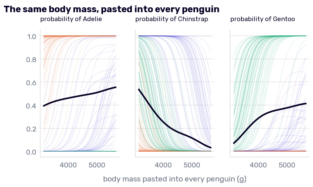
The black curve in the first panel says that a heavier penguin is more likely an Adelie. The table above says that the Adelies are the lightest species. The curve isn’t lying about the model: with the bill and the flipper held where they are, more mass moves a bird from “Chinstrap” to “Adelie”. Read as a fact about penguins, it’s wrong. We met this in Reading the coefficients, where “all else equal” added 1,000 lbs to a car without touching its engine.
The thin curves show who paid for the average. On the left of the middle panel, most of the green curves start above 0.5: the model calls a Gentoo “Chinstrap” once it weighs 3150 g, and the lightest real Gentoo weighs 3950 g. If you plot partial dependence, plot the single curves under it and mark where the real data ends.
LIME
The third tool answers the question differently. LIME2 (local interpretable model-agnostic explanations) says: whatever the model is, close to one row it probably behaves like a line. So draw random rows around the penguin, ask the model about each, give the close ones more weight, and fit a small linear model to the answers. Its coefficients are the explanation.
The lime package had its last release in 2020, and the method fits in a few lines, so I wrote them:
from sklearn.linear_model import Ridge

def lime(width, draws=5000):
    rng = np.random.default_rng(0)
    steps = rng.normal(size=(draws, 4))
    nearby = pd.DataFrame(her.values + steps * model[0].scale_, columns=numeric)
    answers = model.predict_proba(nearby)[:, 0]
    closeness = np.sqrt(np.exp(-(steps ** 2).sum(axis=1) / width ** 2))
    return pd.Series(Ridge(alpha=1).fit(steps, answers, sample_weight=closeness).coef_, index=numeric)
The steps are in standard deviations, the answers are the probabilities of “Adelie”, and width decides how fast the weight of a row falls with its distance from her. The weights, the Ridge, and the 5,000 draws are the package’s defaults.
Again, we know the right answer. The probability has a formula, so its slope at row 172 has one too3:
her_shares = model.predict_proba(her)[0]
true_slope = her_shares[0] * (coefficients.loc['Adelie'] - her_shares @ coefficients.values)
scaled = model[0].transform(seen[numeric])
one_line = Ridge(alpha=1).fit(scaled, model.predict_proba(seen[numeric])[:, 0]).coef_

pd.DataFrame({
    'the true slope at row 172': true_slope,
    **{f'LIME, width {width}': lime(width) for width in [0.5, 1.5, 10]},
    'one line through all 219 penguins': pd.Series(one_line, index=numeric),
}).T.round(2)
| culmen_length_mm | culmen_depth_mm | flipper_length_mm | body_mass_g | |
|---|---|---|---|---|
| the true slope at row 172 | -1.37 | 0.45 | -0.16 | 0.73 |
| LIME, width 0.5 | -0.61 | 0.22 | -0.07 | 0.33 |
| LIME, width 1.5 | -0.39 | 0.15 | -0.06 | 0.19 |
| LIME, width 10 | -0.33 | 0.13 | -0.06 | 0.16 |
| one line through all 219 penguins | -0.37 | 0.17 | -0.11 | 0.12 |
LIME gets the order of the columns and the signs right at every width. The sizes are another matter. For the bill length, the best of them is less than half of the true −1.37.
With a wide kernel, far rows count, and far from her the probability is flat at 0 or 1, so the line gets flatter. A width of 1.5 is the package’s default for four columns (0.75 times the square root of their number). It returns −0.39, and one line fitted through all 219 penguins has −0.37. So at the default, the “local” explanation is mostly the global one. The width is a setting that changes the explanation, and on a real model you have no first row to check it against.
The package differs from my few lines in one more way: by default, it cuts every numeric column into four bins first, so its explanation reads something like “flipper below 190 mm” where mine gives a slope. I’m not claiming my numbers are the ones it would print. The dependence on the width comes with the method.
Every penguin at once
Explanations of single rows can be added up into an explanation of the model. The usual way is to average the absolute Shapley values of many rows per column. I do it for the 54 penguins of her fold, which the model has never seen, add up the three species, and put the permutation importance next to it:
unseen = train_df.drop(index=seen.index)
values = explainer(unseen[numeric]).values
pd.DataFrame({
    'mean absolute Shapley value': pd.DataFrame(np.abs(values).mean(axis=0).sum(axis=1), index=numeric)[0],
    'permutation importance': fold_importance(logistic_with(10))['mean'],
}).round(3)
| mean absolute Shapley value | permutation importance | |
|---|---|---|
| culmen_length_mm | 0.594 | 0.343 |
| culmen_depth_mm | 0.393 | 0.141 |
| flipper_length_mm | 0.204 | 0.036 |
| body_mass_g | 0.381 | 0.132 |
The two columns measure different things and give the same order: bill length, bill depth, body mass, flipper. For the question about the whole model, the tool we have had since Debugging regression model parameters was enough.
What an explanation can’t tell you
Every number in this chapter describes the model. The terms say what the model did with row 172’s measurements, and they are exact. They don’t say what she is. She is a Chinstrap, and the most faithful explanation in the world explains a wrong answer.
My professor’s story from Debugging regression model parameters is the same thing at a larger scale. His team’s model had learned that surgeries by Mr. X on a Monday afternoon end in complications. Any method from this chapter, run on one of those patients, would report the surgeon and the day as the reasons for the prediction, and it would be right about the model. It took the doctors to say that Mr. X was a terrible surgeon every day of the week. An explanation tool shows what the model leans on. Whether that makes sense is still a question for somebody who knows the penguins, or the patients (Rule 12).
All through the chapter, I compared row 172 with groups: all the penguins, the Adelies, the Chinstraps. Those groups came from the species column. In Regression evaluation metrics, I admitted in a footnote that I hadn’t shown you how to find groups of similar rows when no column names them. In the next chapter, I will.
-
Scott Lundberg and Su-In Lee, A Unified Approach to Interpreting Model Predictions, 2017. ↩
-
Marco Tulio Ribeiro, Sameer Singh, and Carlos Guestrin, “Why Should I Trust You?”: Explaining the Predictions of Any Classifier, 2016. ↩
-
Differentiating the formula for \(p_k\) from Logistic regression by one standardized column gives the probability of “Adelie” times the difference between Adelie’s coefficient and the average of the three coefficients, weighted by the three probabilities. ↩